Domain coloring
In mathematics, domain coloring or a color wheel graph is a technique for visualizing complex functions, which assigns a color to each point of the complex plane.
Motivation: four dimensions
A graph of a real function can be drawn in two dimensions, such as x and y. By contrast, a graph of a complex function (more precisely, a complex-valued function of one complex variable f : ℂ → ℂ) requires the visualization of four dimensions. One way to achieve that is with a Riemann surface, another by domain coloring.
Method
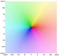
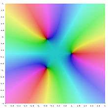
For easy visibility, complex values are represented with colors. This assignment is called a "color function". There are many different color functions used. A common practice is to represent the complex argument (also known as "phase" or "angle") with a hue following the color wheel, and the magnitude by other means, such as brightness or saturation.
Simple color function
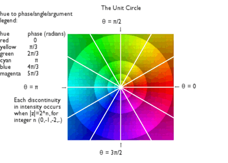
The following example colors the origin in black, 1 in red, −1 in cyan, and a point at infinity in white:

where .

More precisely, it uses the HLS (hue, lightness, saturation) color model. Saturation is always set at the maximum of 100%. Vivid colors of the rainbow are rotating in a continuous way on the complex unit circle, so the sixth roots of unity (starting with 1) are: red, yellow, green, cyan, blue, and magenta. Magnitude is coded by intensity via a strictly monotonic continuous function.
Since the HSL color space is not perceptually uniform, one can see streaks of perceived brightness at yellow, cyan, and magenta (even though their absolute values are the same as red, green, and blue) and a halo around L = 1/2. Use of the Lab color space corrects this, making the images more accurate, but also makes them more drab/pastel.
A structured color function
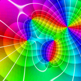
The magnitude of a real number can range from 0 to ∞, a much wider range than that of the argument. Therefore, in a strictly monotonic continuous function that stretches the whole range compromises the resolution of smaller changes in magnitude. This can be achieved with a discontinuous color function, such as the following, which shows a repeating pattern for the magnitude.
In addition, this color function shows white rays for arguments 0, π/6, π/3, π/2, 2π/3, 5π/6, π, 7π/6, 4π/3, 3π/2, 5π/3, 11π/6 and a gray grid for equal real and imaginary values. A similar color function has been used for the graph on top of the article.
History
The method was probably first used in publication in the late 1980s by Larry Crone and Hans Lundmark.[1]
The term "domain coloring" was coined by Frank Farris, possibly around 1998.[2][3] There were many earlier uses of color to visualize complex functions, typically mapping argument (phase) to hue.[4] The technique of using continuous color to map points from domain to codomain or image plane was used in 1999 by George Abdo and Paul Godfrey[5] and colored grids were used in graphics by Doug Arnold that he dates to 1997.[6]
Limitations
People who suffer color blindness may have trouble interpreting such graphs.
References
- ↑ Elias Wegert (2012). Visual Complex Functions: An Introduction with Phase Portraits. Springer Basel. p. 29. ISBN 9783034801799. Retrieved 6 January 2016.
- ↑ Frank A. Farris, Visualizing complex-valued functions in the plane
- ↑ Hans Lundmark (2004). "Visualizing complex analytic functions using domain coloring". Archived from the original on 2006-05-02. Retrieved 2006-05-25. Ludmark refers to Farris' coining the term "domain coloring" in this 2004 article.
- ↑ David A. Rabenhorst (1990). "A Color Gallery of Complex Functions". Pixel: the magazine of scientific visualization. Pixel Communications. 1 (4): 42 et seq.
- ↑ George Abdo & Paul Godfrey (1999). "Plotting functions of a complex variable: Table of Conformal Mappings Using Continuous Coloring". Retrieved 2008-05-17.
- ↑ Douglas N. Arnold (2008). "Graphics for complex analysis". Retrieved 2008-05-17.
External links
- Color Graphs of Complex Functions
- Visualizing complex-valued functions in the plane.
- Gallery of Complex Functions
- Complex Mapper by Alessandro Rosa
- John Davis software − S-Lang script for Domain Coloring
- Open source C and Python domain coloring software
- Enhanced 3D Domain coloring
- Domain Coloring Method on GPU
- Java domain coloring software (In development)
- MATLAB routines
- Python script for GIMP by Michael J. Gruber
- Matplotlib and MayaVi implementation of domain coloring by E. Petrisor
- MATLAB routines with user interface and various color schemes
- MATLAB routines for 3D-visualization of complex functions
- Color wheel method
- Real-Time Zooming Math Engine
- Fractal Zoomer : Software that utilizes domain coloring