Fractional factorial design
In statistics, fractional factorial designs are experimental designs consisting of a carefully chosen subset (fraction) of the experimental runs of a full factorial design [1]. The subset is chosen so as to exploit the sparsity-of-effects principle to expose information about the most important features of the problem studied, while using a fraction of the effort of a full factorial design in terms of experimental runs and resources.
Notation
Fractional designs are expressed using the notation lk − p, where l is the number of levels of each factor investigated, k is the number of factors investigated, and p describes the size of the fraction of the full factorial used. Formally, p is the number of generators, assignments as to which effects or interactions are confounded, i.e., cannot be estimated independently of each other (see below). A design with p such generators is a 1/(lp) fraction of the full factorial design.
For example, a 25 − 2 design is 1/4 of a two level, five factor factorial design. Rather than the 32 runs that would be required for the full 25 factorial experiment, this experiment requires only eight runs.
In practice, one rarely encounters l > 2 levels in fractional factorial designs, since response surface methodology is a much more experimentally efficient way to determine the relationship between the experimental response and factors at multiple levels. In addition, the methodology to generate such designs for more than two levels is much more cumbersome.
The levels of a factor are commonly coded as +1 for the higher level, and −1 for the lower level. For a three-level factor, the intermediate value is coded as 0.
To save space, the points in a two-level factorial experiment are often abbreviated with strings of plus and minus signs. The strings have as many symbols as factors, and their values dictate the level of each factor: conventionally, for the first (or low) level, and for the second (or high) level. The points in this experiment can thus be represented as , , , and .


The factorial points can also be abbreviated by (1), a, b, and ab, where the presence of a letter indicates that the specified factor is at its high (or second) level and the absence of a letter indicates that the specified factor is at its low (or first) level (for example, "a" indicates that factor A is on its high setting, while all other factors are at their low (or first) setting). (1) is used to indicate that all factors are at their lowest (or first) values.
Generation
In practice, experimenters typically rely on statistical reference books to supply the "standard" fractional factorial designs, consisting of the principal fraction. The principal fraction is the set of treatment combinations for which the generators evaluate to + under the treatment combination algebra. However, in some situations, experimenters may take it upon themselves to generate their own fractional design.
A fractional factorial experiment is generated from a full factorial experiment by choosing an alias structure. The alias structure determines which effects are confounded with each other. For example, the five factor 25 − 2 can be generated by using a full three factor factorial experiment involving three factors (say A, B, and C) and then choosing to confound the two remaining factors D and E with interactions generated by D = A*B and E = A*C. These two expressions are called the generators of the design. So for example, when the experiment is run and the experimenter estimates the effects for factor D, what is really being estimated is a combination of the main effect of D and the two-factor interaction involving A and B.
An important characteristic of a fractional design is the defining relation, which gives the set of interaction columns equal in the design matrix to a column of plus signs, denoted by I. For the above example, since D = AB and E = AC, then ABD and ACE are both columns of plus signs, and consequently so is BDCE. In this case the defining relation of the fractional design is I = ABD = ACE = BCDE. The defining relation allows the alias pattern of the design to be determined.
| Treatment combination | I | A | B | C | D = AB | E = AC |
|---|---|---|---|---|---|---|
| de | + | − | − | − | + | + |
| a | + | + | − | − | − | − |
| be | + | − | + | − | − | + |
| abd | + | + | + | − | + | − |
| cd | + | − | − | + | + | − |
| ace | + | + | − | + | − | + |
| bc | + | − | + | + | − | − |
| abcde | + | + | + | + | + | + |
Resolution
An important property of a fractional design is its resolution or ability to separate main effects and low-order interactions from one another. Formally, the resolution of the design is the minimum word length in the defining relation excluding (1). The most important fractional designs are those of resolution III, IV, and V: Resolutions below III are not useful and resolutions above V are wasteful in that the expanded experimentation has no practical benefit in most cases—the bulk of the additional effort goes into the estimation of very high-order interactions which rarely occur in practice. The 25 − 2 design above is resolution III since its defining relation is I = ABD = ACE = BCDE.
| Resolution | Ability | Example |
|---|---|---|
| I | Not useful: an experiment of exactly one run only tests one level of a factor and hence can't even distinguish between the high and low levels of that factor | 21 − 1 with defining relation I = A |
| II | Not useful: main effects are confounded with other main effects | 22 − 1 with defining relation I = AB |
| III | Estimate main effects, but these may be confounded with two-factor interactions | 23 − 1 with defining relation I = ABC |
| IV |
Estimate main effects unconfounded by two-factor interactions |
24 − 1 with defining relation I = ABCD |
| V |
Estimate main effects unconfounded by three-factor (or less) interactions |
25 − 1 with defining relation I = ABCDE |
| VI |
Estimate main effects unconfounded by four-factor (or less) interactions |
26 − 1 with defining relation I = ABCDEF |
The resolution described is only used for regular designs. Regular designs have run size that equal a power of two, and only full aliasing is present. Nonregular designs are designs where run size is a multiple of 4; these designs introduce partial aliasing, and generalized resolution is used as design criterion instead of the resolution described previously.
Example fractional factorial experiment
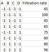
Montgomery [2] gives the following example of a fractional factorial experiment. An engineer performed an experiment to increase the filtration rate (output) of a process to produce a chemical, and to reduce the amount of formaldehyde used in the process. The full factorial experiment is described in the Wikipedia page Factorial experiment. Four factors were considered: temperature (A), pressure (B), formaldehyde concentration (C), and stirring rate (D). The results in that example were that the main effects A, C, and D and the AC and AD interactions were significant. The results of that example may be used to simulate a fractional factorial experiment using a half-fraction of the original 24 = 16 run design. The table shows the 24-1 = 8 run half-fraction experiment design and the resulting filtration rate, extracted from the table for the full 16 run factorial experiment.
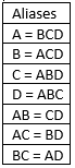
In this fractional design, each main effect is aliased with a 3-factor interaction (e.g., A = BCD), and every 2-factor interaction is aliased with another 2-factor interaction (e.g., AB = CD). The aliasing relationships are shown in the table. This is a resolution IV design, meaning that main effects are aliased with 3-way interactions, and 2-way interactions are aliased with 2-way interactions.
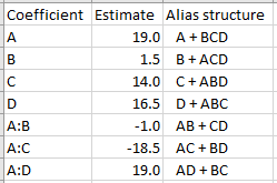
The analysis of variance estimates of the effects are shown in the table below. From inspection of the table, there appear to be large effects due to A, C, and D. The coefficient for the AB interaction is quite small. Unless the AB and CD interactions have approximately equal but opposite effects, these two interactions appear to be negligible. If A, C, and D have large effects, but B has little effect, then the AC and AD interactions are most likely significant. These conclusions are consistent with the results of the full-factorial 16-run experiment.
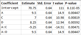
Because B and its interactions appear to be insignificant, B may be dropped from the model. Dropping B results in a full factorial 23 design for the factors A, C, and D. Performing the anova using factors A, C, and D, and the interaction terms A:C and A:D, gives the results shown in the table, which are very similar to the results for the full factorial experiment experiment, but have the advantage of requiring only a half-fraction 8 runs rather than 16.
External links
See also
References
| |||||||||||||||||||||||||||
| |||||||||||||||||||||||||||
| |||||||||||||||||||||||||||
| |||||||||||||||||||||||||||
| |||||||||||||||||||||||||||
| |||||||||||||||||||||||||||
| |||||||||||||||||||||||||||