Financial economics
| Part of a series on |
| Economics |
|---|
 |
|
|
|
By application |
|
Notable economists |
|
Lists |
|
Glossary |
|
Financial economics is the branch of economics characterized by a "concentration on monetary activities", in which "money of one type or another is likely to appear on both sides of a trade".[1] Its concern is thus the interrelation of financial variables, such as prices, interest rates and shares, as opposed to those concerning the real economy. It has two main areas of focus:[2] asset pricing (or "investment theory") and corporate finance; the first being the perspective of providers of capital, i.e. investors, and the second of users of capital.
The subject is concerned with "the allocation and deployment of economic resources, both spatially and across time, in an uncertain environment".[3] It therefore centers on decision making under uncertainty in the context of the financial markets, and the resultant economic and financial models and principles, and is concerned with deriving testable or policy implications from acceptable assumptions. It is built on the foundations of microeconomics and decision theory.
Financial econometrics is the branch of financial economics that uses econometric techniques to parameterise these relationships. Mathematical finance is related in that it will derive and extend the mathematical or numerical models suggested by financial economics. Note though that the emphasis there is mathematical consistency, as opposed to compatibility with economic theory. Financial economics has a primarily microeconomic focus, whereas monetary economics is primarily macroeconomic in nature.
Financial economics is usually taught at the postgraduate level; see Master of Financial Economics. Recently, specialist undergraduate degrees are offered in the discipline.[4]
This article provides an overview and survey of the field: for derivations and more technical discussion, see the specific articles linked.
Underlying economics
| JEL classification codes |
| In the Journal of Economic Literature classification codes, Financial Economics is one of the 19 primary classifications, at JEL: G. It follows Monetary and International Economics and precedes Public Economics. For detailed subclassifications see JEL classification codes § G. Financial Economics.
The New Palgrave Dictionary of Economics (2008, 2nd ed.) also uses the JEL codes to classify its entries in v. 8, Subject Index, including Financial Economics at pp. 863–64. The below have links to entry abstracts of The New Palgrave Online for each primary or secondary JEL category (10 or fewer per page, similar to Google searches):
Tertiary category entries can also be searched.[5] |
As above, the discipline essentially explores how rational investors would apply decision theory to the problem of investment. The subject is thus built on the foundations of microeconomics and decision theory, and derives several key results for the application of decision making under uncertainty to the financial markets.
Present value, expectation and utility
Underlying all of financial economics are the concepts of present value and expectation.[6]
Calculating their present value allows the decision maker to aggregate the cashflows (or other returns) to be produced by the asset in the future, to a single value at the date in question, and to thus more readily compare two opportunities; this concept is therefore the starting point for financial decision making. (Its history is correspondingly early: Richard Witt discusses compound interest in depth already in 1613, in his book "Arithmeticall Questions";[7] further developed by Johan de Witt and Edmond Halley.)
An immediate extension is to combine probabilities with present value, leading to the expected value criterion which sets asset value as a function of the sizes of the expected payouts and the probabilities of their occurrence. (These ideas originate with Blaise Pascal and Pierre de Fermat.)
This decision method, however, fails to consider risk aversion ("as any student of finance knows"[6]). In other words, since individuals receive greater utility from an extra dollar when they are poor and less utility when comparatively rich, the approach is to therefore "adjust" the weight assigned to the various outcomes ("states") correspondingly. (Some investors may in fact be risk seeking as opposed to risk averse, but the same logic would apply).
Choice under uncertainty here may then be characterized as the maximization of expected utility. More formally, the resulting expected utility hypothesis states that, if certain axioms are satisfied, the subjective value associated with a gamble by an individual is that individual's statistical expectation of the valuations of the outcomes of that gamble.
The impetus for these ideas arise from various inconsistencies observed under the expected value framework, such as the St. Petersburg paradox; see also Ellsberg paradox. (The development here is originally due to Daniel Bernoulli, and later formalized by John von Neumann and Oskar Morgenstern.)
Arbitrage-free pricing and equilibrium
The concepts of arbitrage-free, "rational", pricing and equilibrium are then coupled with the above to derive "classical"[8] (or "neo-classical"[9]) financial economics.
Rational pricing is the assumption that asset prices (and hence asset pricing models) will reflect the arbitrage-free price of the asset, as any deviation from this price will be "arbitraged away". This assumption is useful in pricing fixed income securities, particularly bonds, and is fundamental to the pricing of derivative instruments.
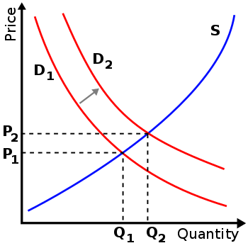
Economic equilibrium is, in general, a state in which economic forces such as supply and demand are balanced, and, in the absence of external influences these equilibrium values of economic variables will not change. General equilibrium deals with the behavior of supply, demand, and prices in a whole economy with several or many interacting markets, by seeking to prove that a set of prices exists that will result in an overall equilibrium. (This is in contrast to partial equilibrium, which only analyzes single markets.)
The two concepts are linked as follows: where market prices do not allow for profitable arbitrage, i.e. they comprise an arbitrage-free market, then these prices are also said to constitute an "arbitrage equilibrium". Intuitively, this may be seen by considering that where an arbitrage opportunity does exist, then prices can be expected to change, and are therefore not in equilibrium.[10] An arbitrage equilibrium is thus a precondition for a general economic equilibrium.
The immediate, and formal, extension of this idea, the fundamental theorem of asset pricing, shows that where markets are as described —and are additionally (implicitly and correspondingly) complete—one may then make financial decisions by constructing a risk neutral probability measure corresponding to the market.
"Complete" here means that there is a price for every asset in every possible state of the world, and that the complete set of possible bets on future states-of-the-world can therefore be constructed with existing assets (assuming no friction), essentially solving simultaneously for n (risk-neutral) probabilities, given n prices. The formal derivation will proceed by arbitrage arguments.[6][10] For a worked example see Rational pricing#Risk neutral valuation, where, in a simplified environment, the economy has only two possible states—up and down—and where p and (1−p) are the two corresponding (i.e. implied) probabilities, and in turn, the derived distribution, or "measure".
With this measure in place, the expected, i.e. required, return of any security (or portfolio) will then equal the riskless return, plus an "adjustment for risk",[6] i.e. a security-specific risk premium, compensating for the extent to which its cashflows are unpredictable. All pricing models are then essentially variants of this, given specific assumptions and/or conditions.[6][11] This approach is consistent with the above, but with the expectation based on "the market" (i.e. arbitrage-free, and, per the theorem, therefore in equilibrium) as opposed to individual preferences.
Thus, continuing the example, to value a specific security, its forecasted cashflows in the up- and down-states are multiplied through by p and (1-p) respectively, and are then discounted at the risk-free interest rate plus an appropriate premium. In general, this premium may be derived by the CAPM (or extensions) as will be seen under #Uncertainty.
State prices
With the above relationship established, the further specialized Arrow–Debreu model may be derived. This important result suggests that, under certain economic conditions, there must be a set of prices such that aggregate supplies will equal aggregate demands for every commodity in the economy. The analysis here is often undertaken assuming a representative agent.[12]
The Arrow–Debreu model applies to economies with maximally complete markets, in which there exists a market for every time period and forward prices for every commodity at all time periods. A direct extension, then, is the concept of a state price security (also called an Arrow–Debreu security), a contract that agrees to pay one unit of a numeraire (a currency or a commodity) if a particular state occurs ("up" and "down" in the simplified example above) at a particular time in the future and pays zero numeraire in all the other states. The price of this security is the state price of this particular state of the world.
In the above example, the state prices would equate to the present values of $p and $(1−p): i.e. what one would pay today, respectively, for the up- and down-state securities; the state price vector is the vector of state prices for all states. Applied to valuation, the price of the derivative today would simply be [up-state-price × up-state-payoff + down-state-price × down-state-payoff]; see below regarding the absence of any risk premium here. For a continuous random variable indicating a continuum of possible states, the value is found by integrating over the state price density; see Stochastic discount factor. These concepts are extended to martingale pricing and the related risk-neutral measure.
State prices find immediate application as a conceptual tool ("contingent claim analysis");[6] but can also be applied to valuation problems.[13] Given the pricing mechanism described, one can decompose the derivative value (true in fact for "every security" [2]) as a linear combination of its state-prices; i.e. back-solve for the state-prices corresponding to observed derivative prices.[14][13] These recovered state-prices can then be used for valuation of other instruments with exposure to the underlyer, or for other decision making relating to the underlyer itself. (Breeden and Litzenberger's work in 1978 [15] established the use of state prices in financial economics.)
Resultant models

| The capital asset pricing model (CAPM)
|

| The Black–Scholes equation
|

| The Black–Scholes formula for the value of a call option:
Interpretation: is the probability that the call will be exercised; is the present value of the expected asset price at expiration, given that the asset price at expiration is above the exercise price. |
![{\begin{aligned}C(S,t)&=N(d_{1})S-N(d_{2})Ke^{-r(T-t)}\\d_{1}&={\frac {1}{\sigma {\sqrt {T-t}}}}\left[\ln \left({\frac {S}{K}}\right)+\left(r+{\frac {\sigma ^{2}}{2}}\right)(T-t)\right]\\d_{2}&=d_{1}-\sigma {\sqrt {T-t}}\\\end{aligned}}](../I/m/f6ed0aef39b1aee3a602de0faf6224848c506363.svg)


Applying the preceding economic concepts, we may then derive various economic- and financial models and principles. As above, the two usual areas of focus are Asset Pricing and Corporate Finance, the first being the perspective of providers of capital, the second of users of capital. Here, and for (almost) all other financial economics models, the questions addressed are typically framed in terms of "time, uncertainty, options, and information",[1][12] as will be seen below.
- Time: money now is traded for money in the future.
- Uncertainty (or risk): The amount of money to be transferred in the future is uncertain.
- Options: one party to the transaction can make a decision at a later time that will affect subsequent transfers of money.
- Information: knowledge of the future can reduce, or possibly eliminate, the uncertainty associated with future monetary value (FMV).
Applying this framework, with the above concepts, leads to the required models. This derivation begins with the assumption of "no uncertainty" and is then expanded to incorporate the other considerations. (This division sometimes denoted "deterministic" and "random",[16] or "stochastic".)
Certainty
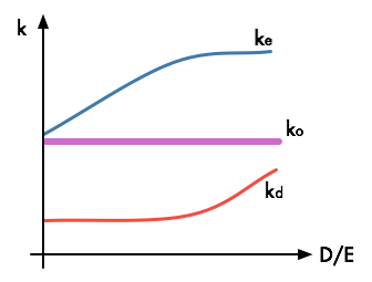
The starting point here is “Investment under certainty". The Fisher separation theorem, asserts that the objective of a corporation will be the maximization of its present value, regardless of the preferences of its shareholders. Related is the Modigliani–Miller theorem, which shows that, under certain conditions, the value of a firm is unaffected by how that firm is financed, and depends neither on its dividend policy nor its decision to raise capital by issuing stock or selling debt. The proof here proceeds using arbitrage arguments, and acts as a benchmark for evaluating the effects of factors outside the model that do affect value.
The mechanism for determining (corporate) value is provided by The Theory of Investment Value (John Burr Williams), which proposes that the value of an asset should be calculated using "evaluation by the rule of present worth". Thus, for a common stock, the intrinsic, long-term worth is the present value of its future net cashflows, in the form of dividends. What remains to be determined is the appropriate discount rate. Later developments show that, "rationally", i.e. in the formal sense, the appropriate discount rate here will (should) depend on the asset's riskiness relative to the overall market, as opposed to its owners' preferences; see below. Net present value (NPV) is the direct extension of these ideas typically applied to Corporate Finance decisioning (introduced by Joel Dean in 1951). For other results, as well as specific models developed here, see the list of "Equity valuation" topics under Outline of finance#Discounted cash flow valuation.
Bond valuation, in that cashflows (coupons and return of principal) are deterministic, may proceed in the same fashion.[16] An immediate extension, Arbitrage-free bond pricing, discounts each cashflow at the market derived rate — i.e. at each coupon's corresponding zero-rate — as opposed to an overall rate. Note that in many treatments bond valuation precedes equity valuation, under which cashflows (dividends) are not "known" per se. Williams and onward allow for forecasting as to these — based on historic ratios or published policy — and cashflows are then treated as essentially deterministic; see below under #Corporate finance theory.
These "certainty" results are all commonly employed under corporate finance; uncertainty is the focus of "asset pricing models", as follows.
Uncertainty
For "choice under uncertainty" the twin assumptions of rationality and market efficiency, as more closely defined, lead to modern portfolio theory (MPT) with its capital asset pricing model (CAPM)—an equilibrium-based result—and to the Black–Scholes–Merton theory (BSM; often, simply Black–Scholes) for option pricing—an arbitrage-free result. Note that the latter derivative prices are calculated such that they are arbitrage-free with respect to the more fundamental, equilibrium determined, securities prices; see asset pricing.
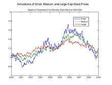
Briefly, and intuitively—and consistent with #Arbitrage-free pricing and equilibrium above—the linkage is as follows.[17] Given the ability to profit from private information, self-interested traders are motivated to acquire and act on their private information. In doing so, traders contribute to more and more "correct", i.e. efficient, prices: the efficient-market hypothesis, or EMH (Eugene Fama, 1965). The EMH (implicitly) assumes that average expectations constitute an "optimal forecast", i.e. prices using all available information, are identical to the best guess of the future: the assumption of rational expectations. The EMH does allow that when faced with new information, some investors may overreact and some may underreact, but what is required, however, is that investors' reactions follow a normal distribution—so that the net effect on market prices cannot be reliably exploited to make an abnormal profit. In the competitive limit, then, market prices will reflect all available information and prices can only move in response to news;[18] and this, of course, could be "good" or "bad", major or minor: the random walk hypothesis. Thus, if prices of financial assets are (broadly) efficient, then deviations from these (equilibrium) values could not last for long. (On Random walks in stock prices: Jules Regnault, 1863; Louis Bachelier, 1900; Maurice Kendall, 1953; Paul Cootner, 1964.)
Under these conditions investors can then be assumed to act rationally: their investment decision must be calculated or a loss is sure to follow; correspondingly, where an arbitrage opportunity presents itself, then arbitrageurs will exploit it, reinforcing this equilibrium. Here, as under the certainty-case above, the specific assumption as to pricing is that prices are calculated as the present value of expected future dividends,[11][18][12] as based on currently available information. What is required though is a theory for determining the appropriate discount rate, i.e. "required return", given this uncertainty: this is provided by the MPT and its CAPM. Relatedly, rationality—in the sense of arbitrage-exploitation—gives rise to Black–Scholes; option values here ultimately consistent with the CAPM.
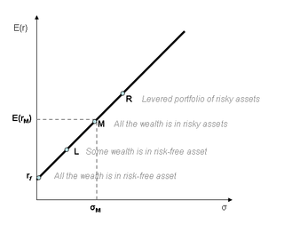
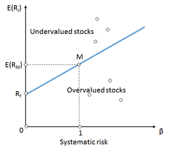
In general, then, while portfolio theory studies how investors should balance risk and return when investing in many assets or securities, the CAPM is more focused, describing how, in equilibrium, markets set the prices of assets in relation to how risky they are. Importantly, this result will be independent of the investor's level of risk aversion, and / or assumed utility function, thus providing a readily determined discount rate for corporate finance decision makers as above,[19] and for other investors. The argument proceeds as follows: If one can construct an efficient frontier—i.e. each combination of assets offering the best possible expected level of return for its level of risk, see diagram—then mean-variance efficient portfolios can be formed simply as a combination of holdings of the risk-free asset and the "market portfolio" (the Mutual fund separation theorem), with the combinations here plotting as the capital market line, or CML. Then, given this CML, the required return on risky securities will be independent of the investor's utility function, and solely determined by their covariance ("beta") with aggregate, i.e. market, risk. This is because investors here can then maximize utility through leverage as opposed to pricing; see CML diagram. As can be seen in the formula aside, this result is consistent with the preceding, equaling the riskless return plus an adjustment for risk.[11] (The efficient frontier was introduced by Harry Markowitz in 1952. The CAPM was derived by Jack Treynor (1961, 1962), William F. Sharpe (1964), John Lintner (1965) and Jan Mossin (1966) independently.)
Black–Scholes provides a mathematical model of a financial market containing derivative instruments, and the resultant formula for the price of European-styled options. The model is expressed as the Black–Scholes equation, a partial differential equation describing the changing price of the option over time; it is derived assuming log-normal, geometric Brownian motion (see Brownian model of financial markets). The key financial insight behind the model is that one can perfectly hedge the option by buying and selling the underlying asset in just the right way and consequently "eliminate risk", absenting the risk adjustment from the pricing ( , the value, or price, of the option, grows at , the risk-free rate; see Black–Scholes equation § Financial interpretation).[6][11] This hedge, in turn, implies that there is only one right price—in an arbitrage-free sense—for the option. And this price is returned by the Black–Scholes option pricing formula. (The formula, and hence the price, is consistent with the equation, as the formula is the solution to the equation.) Since the formula is without reference to the share's expected return, Black–Scholes entails (assumes) risk neutrality, consistent with the "elimination of risk" here. Relatedly, therefore, the pricing formula may also be derived directly via risk neutral expectation. (BSM - two seminal 1973 papers [20] [21] - is consistent with "previous versions of the formula" of Louis Bachelier and Edward O. Thorp;[22] although these were more "actuarial" in flavor, and had not established risk-neutral discounting.[9] See also Paul Samuelson (1965).[23] Vinzenz Bronzin (1908) produced very early results.)


As mentioned, it can be shown that the two models are consistent; then, as is to be expected, "classical" financial economics is thus unified. Here, the Black Scholes equation may alternatively be derived from the CAPM, and the price obtained from the Black–Scholes model is thus consistent with the expected return from the CAPM.[24][9] The Black–Scholes theory, although built on Arbitrage-free pricing, is therefore consistent with the equilibrium based capital asset pricing. Both models, in turn, are ultimately consistent with the Arrow–Debreu theory, and may be derived via state-pricing,[6] further explaining, and if required demonstrating, this unity.
Extensions
More recent work further generalizes and / or extends these models. As regards asset pricing, developments in equilibrium-based pricing are discussed under "Portfolio theory" below, while "Derivative pricing" relates to risk-neutral, i.e. arbitrage-free, pricing. As regards the use of capital, "Corporate finance theory" relates, mainly, to the application of these models.
Portfolio theory

- See also: Post-modern portfolio theory and Mathematical finance § Risk and portfolio management: the P world.
The majority of developments here relate to required return, i.e. pricing, extending the basic CAPM. Multi-factor models such as the Fama–French three-factor model and the Carhart four-factor model, propose factors other than market return as relevant in pricing. The intertemporal CAPM and consumption-based CAPM similarly extend the model. With intertemporal portfolio choice, the investor now repeatedly optimizes her portfolio; while the inclusion of consumption (in the economic sense) then incorporates all sources of wealth, and not just market-based investments, into the investor's calculation of required return.
Whereas the above extend the CAPM, the single-index model is a more simple model. It assumes, only, a correlation between security and market returns, without (numerous) other economic assumptions. It is useful in that it simplifies the estimation of correlation between securities, significantly reducing the inputs for building the correlation matrix required for portfolio optimization. The arbitrage pricing theory (APT; Stephen Ross, 1976) similarly differs as regards its assumptions. APT "gives up the notion that there is one right portfolio for everyone in the world, and ...replaces it with an explanatory model of what drives asset returns."[25] It returns the required (expected) return of a financial asset as a linear function of various macro-economic factors, and assumes that arbitrage should bring incorrectly priced assets back into line.
As regards portfolio optimization, the Black–Litterman model departs from the original Markowitz approach of constructing portfolios via an efficient frontier. Black–Litterman instead starts with an equilibrium assumption, and is then modified to take into account the 'views' (i.e., the specific opinions about asset returns) of the investor in question to arrive at a bespoke asset allocation. Where factors additional to volatility are considered (kurtosis, skew...) then multiple-criteria decision analysis can be applied; here deriving a Pareto efficient portfolio. The universal portfolio algorithm (Thomas M. Cover) applies machine learning to asset selection, learning adaptively from historical data. Behavioral portfolio theory recognizes that investors have varied aims and create an investment portfolio that meets a broad range of goals. Copulas have lately been applied here. See Portfolio optimization § Improving portfolio optimization for other techniques and / or objectives.
Derivative pricing
| PDE for a zero-coupon bond
|
![{\frac {1}{2}}\sigma (r)^{{2}}{\frac {\partial ^{2}P}{\partial r^{2}}}+[a(r)+\sigma (r)+\varphi (r,t)]{\frac {\partial P}{\partial r}}+{\frac {\partial P}{\partial t}}-rP=0](../I/m/ec0f423e539923eb96e77014e6bee05c362cf22d.svg)
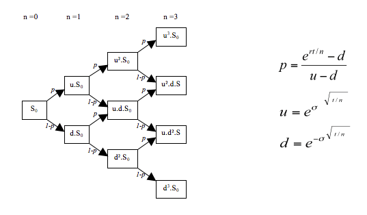
As regards derivative pricing, the binomial options pricing model provides a discretized version of Black–Scholes, useful for the valuation of American styled options. Discretized models of this type are built—at least implicitly—using state-prices (as above); relatedly, a large number of researchers have used options to extract state-prices for a variety of other applications in financial economics.[6][24][14] For path dependent derivatives, Monte Carlo methods for option pricing are employed; here the modelling is in continuous time, but similarly uses risk neutral expected value. Various other numeric techniques have also been developed. The theoretical framework too has been extended such that martingale pricing is now the standard approach. Developments relating to complexities in return and / or volatility are discussed below.
Drawing on these techniques, derivative models for various other underlyings and applications have also been developed, all based off the same logic (using "contingent claim analysis"). Real options valuation allows that option holders can influence the option's underlying; models for employee stock option valuation explicitly assume non-rationality on the part of option holders; Credit derivatives allow that payment obligations and / or delivery requirements might not be honored. Exotic derivatives are now routinely valued. Multi-asset underlyers are handled via simulation or copula based analysis.
Similarly, beginning with Oldrich Vasicek (1977), various short rate models, as well as the HJM and BGM forward rate-based techniques, allow for an extension of these techniques to fixed income- and interest rate derivatives. (The Vasicek and CIR models are equilibrium-based, while Ho–Lee and subsequent models are based on arbitrage-free pricing.) Bond valuation is relatedly extended: the Stochastic calculus approach, employing these methods, allows for rates that are "random" (while returning a price that is arbitrage free, as above); lattice models for hybrid securities allow for non-deterministic cashflows (and stochastic rates).
As above, (OTC) derivative pricing has relied on the BSM risk neutral pricing framework, under the assumptions of funding at the risk free rate and the ability to perfectly replicate cashflows so as to fully hedge. This, in turn, is built on the assumption of a credit-risk-free environment. Post the financial crisis of 2008, therefore, issues such as counterparty credit risk, funding costs and costs of capital are additionally considered,[26] and a Credit Valuation Adjustment, or CVA—and potentially other valuation adjustments, collectively xVA—is generally added to the risk-neutral derivative value.
A related, and perhaps more fundamental change, is that discounting is now on the Overnight Index Swap (OIS) curve, as opposed to LIBOR as used previously. This is because post-crisis, OIS is considered a better proxy for the "risk-free rate".[27] (Also, practically, the interest paid on cash collateral is usually the overnight rate; OIS discounting is then, sometimes, referred to as "CSA discounting".) Swap pricing is further modified: previously, swaps were valued off a single "self discounting" interest rate curve; whereas post crisis, to accommodate OIS discounting, valuation is now under a "multi-curve" framework where "forecast curves" are constructed for each floating-leg LIBOR tenor, with discounting on a common OIS curve; see Interest rate swap § Valuation and pricing.
Corporate finance theory
Corporate finance theory has also been extended: mirroring the above developments, asset-valuation and decisioning no longer need assume "certainty". As discussed, Monte Carlo methods in finance, introduced by David B. Hertz in 1964, allow financial analysts to construct "stochastic" or probabilistic corporate finance models, as opposed to the traditional static and deterministic models;[28] see Corporate finance § Quantifying uncertainty. Relatedly, Real Options theory allows for owner—i.e. managerial—actions that impact underlying value: by incorporating option pricing logic, these actions are then applied to a distribution of future outcomes, changing with time, which then determine the "project's" valuation today.[29]
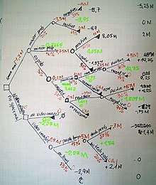
More traditionally, decision trees—which are complementary—have been used to evaluate projects, by incorporating in the valuation (all) possible events (or states) and consequent management decisions;[30][28] the correct discount rate here reflecting each point's "non-diversifiable risk looking forward."[28] (This technique predates the use of real options in corporate finance;[31] it is borrowed from operations research, and is not a "financial economics development" per se.)
Related to this, is the treatment of forecasted cashflows in equity valuation. In many cases, following Williams above, the average (or most likely) cash-flows were discounted,[32] as opposed to a more correct state-by-state treatment under uncertainty; see comments under Financial modeling § Accounting. In more modern treatments, then, it is the expected cashflows (in the mathematical sense) combined into an overall value per forecast period which are discounted.[33][34][35][28] And using the CAPM—or extensions—the discounting here is at the risk-free rate plus a premium linked to the uncertainty of the entity or project cash flows.[28][34]
Other extensions here include[36] agency theory, which analyses the difficulties in motivating corporate management (the "agent") to act in the best interests of shareholders (the "principal"), rather than in their own interests. Clean surplus accounting and the related residual income valuation provide a model that returns price as a function of earnings, expected returns, and change in book value, as opposed to dividends. This approach, to some extent, arises due to the implicit contradiction of seeing value as a function of dividends, while also holding that dividend policy cannot influence value per Modigliani and Miller's "Irrelevance principle"; see Dividend policy § Irrelevance of dividend policy.
The typical application of real options is to capital budgeting type problems as described. However, they are also applied to questions of capital structure and dividend policy, and to the related design of corporate securities; and since stockholder and bondholders have different objective functions, in the analysis of the related agency problems.[29] In all of these cases, state-prices can provide the market-implied information relating to the corporate, as above, which is then applied to the analysis. For example, convertible bonds can (must) be priced consistent with the state-prices of the corporate's equity.[13][33]
Challenges and criticism
As above, there is a very close link between (i) the random walk hypothesis, with the associated expectation that price changes should follow a normal distribution, on the one hand, and (ii) market efficiency and rational expectations, on the other. Note, however, that (wide) departures from these are commonly observed, and there are thus, respectively, two main sets of challenges.
Departures from normality
As discussed, the assumptions that market prices follow a random walk and / or that asset returns are normally distributed are fundamental. Empirical evidence, however, suggests that these assumptions may not hold (see Kurtosis risk, Skewness risk, Long tail) and that in practice, traders, analysts and risk managers frequently modify the "standard models" (see Model risk). In fact, Benoît Mandelbrot had discovered already in the 1960s that changes in financial prices do not follow a Gaussian distribution, the basis for much option pricing theory, although this observation was slow to find its way into mainstream financial economics.
Financial models with long-tailed distributions and volatility clustering have been introduced to overcome problems with the realism of the above "classical" financial models; while jump diffusion models allow for (option) pricing incorporating "jumps" in the spot price.[37] Risk managers, similarly, complement (or substitute) the standard value at risk models with historical simulations, mixture models, principal component analysis, extreme value theory, as well as models for volatility clustering.[38] For further discussion see Fat-tailed distribution § Applications in economics, and Value at risk § Criticism. Portfolio managers, likewise, have modified their optimization criteria and algorithms; see #Portfolio theory above.
Closely related is the volatility smile, where implied volatility—the volatility corresponding to the BSM price—is observed to differ as a function of strike price (i.e. moneyness), true only if the price-change distribution is non-normal, unlike that assumed by BSM. The term structure of volatility describes how (implied) volatility differs for related options with different maturities. An implied volatility surface is then a three-dimensional surface plot of volatility smile and term structure. These empirical phenomena negate the assumption of constant volatility—and log-normality—upon which Black–Scholes is built;[22][37] see Black–Scholes model § The volatility smile.
In consequence traders (and risk managers) use "smile-consistent" models, firstly, when valuing derivatives not directly mapped to the surface, facilitating the pricing of other, i.e. non-quoted, strike/maturity combinations, or of non-European derivatives, and generally for hedging purposes. The two main approaches are local volatility and stochastic volatility. The first returns the volatility which is “local” to each spot-time point of the finite difference- or simulation-based valuation — i.e. as opposed to implied volatility, which holds overall. In this way calculated prices — and numeric structures — are market-consistent in an arbitrage-free sense. The second approach assumes that the volatility of the underlying price is a stochastic process rather than a constant. Models here are first "calibrated" to observed prices, and are then applied to the valuation in question; the most common are Heston, SABR and CEV. This approach addresses certain problems identified with hedging under local volatility.[39]
Related to local volatility are the lattice-based implied-binomial and -trinomial trees — essentially a discretization of the approach — which are similarly used for pricing; these are built on state-prices recovered from the surface. Edgeworth binomial trees allow for a specified (i.e. non-Gaussian) skew and kurtosis in the spot price; priced here, options with differing strikes will return differing implied volatilities, and the tree can be calibrated to the smile as required.[40] Similarly purposed closed-form models have also been developed. [41]
As above, additional to log-normality in returns, BSM—and, typically, other derivative models—assume(d) the ability to perfectly replicate cashflows so as to fully hedge, and hence to discount at the risk-free rate. This, in turn, is built on the assumption of a credit-risk-free environment. Post crisis, then, various x-value adjustments are made to the risk-neutral derivative value. Note that these are additional to any smile or surface effect: this is valid as the surface is built on price data relating to fully collateralized positions, and there is therefore no "double counting" of credit risk (etc.) when including xVA. (Also, were this not the case, then each counterparty would have its own surface...)
Departures from rationality
| Market anomalies and Economic puzzles |
As seen, a common assumption is that financial decision makers act rationally; see Homo economicus. Recently, however, researchers in experimental economics and experimental finance have challenged this assumption empirically. These assumptions are also challenged theoretically, by behavioral finance, a discipline primarily concerned with the limits to rationality of economic agents.
Consistent with, and complementary to these findings, various persistent market anomalies have been documented, these being price and/or return distortions—e.g. size premiums—which appear to contradict the efficient-market hypothesis; calendar effects are the best known group here. Related to these are various of the economic puzzles, concerning phenomena similarly contradicting the theory. The equity premium puzzle, as one example, arises in that the difference between the observed returns on stocks as compared to government bonds is consistently higher than the risk premium rational equity investors should demand, an "abnormal return". For further context see Random walk hypothesis § A non-random walk hypothesis, and sidebar for specific instances.
More generally, and particularly following the financial crisis of 2007–2010, financial economics and mathematical finance have been subjected to deeper criticism; notable here is Nassim Nicholas Taleb, who claims that the prices of financial assets cannot be characterized by the simple models currently in use, rendering much of current practice at best irrelevant, and, at worst, dangerously misleading; see Black swan theory, Taleb distribution. A topic of general interest studied in recent years has thus been financial crises,[42] and the failure of financial economics to model these. (A related problem is systemic risk: where companies hold securities in each other then this interconnectedness may entail a "valuation chain"—and the performance of one company, or security, here will impact all, a phenomenon not easily modeled, regardless of whether the individual models are correct. See Systemic risk § Inadequacy of classic valuation models; Cascades in financial networks; Flight-to-quality.)
Areas of research attempting to explain (or at least model) these phenomena, and crises, include[12] noise trading, market microstructure, and Heterogeneous agent models. The latter is extended to agent-based computational economics, where price is treated as an emergent phenomenon, resulting from the interaction of the various market participants (agents). The noisy market hypothesis argues that prices can be influenced by speculators and momentum traders, as well as by insiders and institutions that often buy and sell stocks for reasons unrelated to fundamental value; see Noise (economic). The adaptive market hypothesis is an attempt to reconcile the efficient market hypothesis with behavioral economics, by applying the principles of evolution to financial interactions. An information cascade, alternatively, shows market participants engaging in the same acts as others ("herd behavior"), despite contradictions with their private information. Copula-based modelling has similarly been applied. See also Hyman Minsky's "financial instability hypothesis", as well as George Soros' approach, § Reflexivity, financial markets, and economic theory.
On the obverse, however, various studies have shown that despite these departures from efficiency, asset prices do typically exhibit a random walk and that one cannot therefore consistently outperform market averages ("alpha").[43] The practical implication, therefore, is that passive investing (e.g. via low-cost index funds) should, on average, serve better than any other active strategy.[44] Burton Malkiel's A Random Walk Down Wall Street—first published in 1973, and in its 11th edition as of 2015—is a widely read popularization of these arguments. (See also John C. Bogle's Common Sense on Mutual Funds; but compare Warren Buffett's The Superinvestors of Graham-and-Doddsville.) Note also that institutionally inherent limits to arbitrage—as opposed to factors directly contradictory to the theory—are sometimes proposed as an explanation for these departures from efficiency.
See also
- Category:Finance theories
- Category:Financial economists
- Deutsche Bank Prize in Financial Economics
- Financial modeling
- Fischer Black Prize
- List of unsolved problems in economics § Financial economics
- Monetary economics
- Outline of economics
- Outline of finance
References
- 1 2 William F. Sharpe, "Financial Economics" Archived 2004-06-04 at the Wayback Machine., in "Macro-Investment Analysis". Stanford University (manuscript). Archived from the original on 2014-07-14. Retrieved 2009-08-06.
- 1 2 Merton H. Miller, (1999). The History of Finance: An Eyewitness Account, Journal of Portfolio Management. Summer 1999.
- ↑ Robert C. Merton "Nobel Lecture" (PDF). Archived (PDF) from the original on 2009-03-19. Retrieved 2009-08-06.
- ↑ e.g.: Kent Archived 2014-02-21 at the Wayback Machine.; City London Archived 2014-02-23 at the Wayback Machine.; UC Riverside Archived 2014-02-22 at the Wayback Machine.; Leicester Archived 2014-02-22 at the Wayback Machine.; Toronto Archived 2014-02-21 at the Wayback Machine.; UMBC Archived 2014-12-30 at the Wayback Machine.
- ↑ For example, http://www.dictionaryofeconomics.com/search_results?q=&field=content&edition=all&topicid=G00 Archived 2013-05-29 at the Wayback Machine..
- 1 2 3 4 5 6 7 8 9 Rubinstein, Mark. (2005). "Great Moments in Financial Economics: IV. The Fundamental Theorem (Part I)", Journal of Investment Management, Vol. 3, No. 4, Fourth Quarter 2005; ~ (2006). Part II, Vol. 4, No. 1, First Quarter 2006. See under "External links".
- ↑ C. Lewin (1970). An early book on compound interest Archived 2016-12-21 at the Wayback Machine., Institute and Faculty of Actuaries
- ↑ See Rubinstein under "Bibliography".
- 1 2 3 Emanuel Derman, A Scientific Approach to CAPM and Options Valuation Archived 2016-03-30 at the Wayback Machine.
- 1 2 Freddy Delbaen and Walter Schachermayer. (2004). "What is... a Free Lunch?" Archived 2016-03-04 at the Wayback Machine. (pdf). Notices of the AMS 51 (5): 526–528
- 1 2 3 4 Christopher L. Culp and John H. Cochrane. (2003). ""Equilibrium Asset Pricing and Discount Factors: Overview and Implications for Derivatives Valuation and Risk Management" Archived 2016-03-04 at the Wayback Machine., in Modern Risk Management: A History. Peter Field, ed. London: Risk Books, 2003. ISBN 1904339050
- 1 2 3 4 Farmer J. Doyne, Geanakoplos John (2009). "The virtues and vices of equilibrium and the future of financial economics" (PDF). Complexity. 14 (3). arXiv:0803.2996. Bibcode:2009Cmplx..14c..11F. doi:10.1002/cplx.20261.
- 1 2 3 See de Matos, as well as Bossaerts and Ødegaard, under bibliography.
- 1 2 Don M. Chance (2008). "Option Prices and State Prices" Archived 2012-02-09 at the Wayback Machine.
- ↑ Breeden, Douglas T.; Litzenberger, Robert H. (1978). "Prices of State-Contingent Claims Implicit in Option Prices". Journal of Business. 51 (4): 621–651. doi:10.1086/296025. JSTOR 2352653.
- 1 2 See Luenberger's Investment Science, under Bibliography.
- ↑ For a more formal treatment, see, for example: Eugene F. Fama. 1965. Random Walks in Stock Market Prices. Financial Analysts Journal, September/October 1965, Vol. 21, No. 5: 55–59.
- 1 2 Shiller, Robert J. (2003). "From Efficient Markets Theory to Behavioral Finance" (PDF). Journal of Economic Perspectives. 17 (1 (Winter 2003)): 83–104. doi:10.1257/089533003321164967. Archived (PDF) from the original on 2015-04-12.
- ↑ Jensen, Michael C. and Smith, Clifford W., "The Theory of Corporate Finance: A Historical Overview". In: The Modern Theory of Corporate Finance, New York: McGraw-Hill Inc., pp. 2–20, 1984.
- ↑ Black, Fischer; Myron Scholes (1973). "The Pricing of Options and Corporate Liabilities". Journal of Political Economy. 81 (3): 637–654. doi:10.1086/260062.
- ↑ Merton, Robert C. (1973). "Theory of Rational Option Pricing". Bell Journal of Economics and Management Science. The RAND Corporation. 4 (1): 141–183. doi:10.2307/3003143. JSTOR 3003143.
- 1 2 Haug, E. G. and Taleb, N. N. (2008): Why We Have Never Used the Black-Scholes-Merton Option Pricing Formula Archived 2011-05-03 at the Wayback Machine., Wilmott Magazine January 2008
- ↑ Samuelson Paul (1965). "A Rational Theory of Warrant Pricing" (PDF). Industrial Management Review. 6: 2. Archived (PDF) from the original on 2017-03-01. Retrieved 2017-02-28.
- 1 2 Don M. Chance (2008). "Option Prices and Expected Returns" Archived 2015-09-23 at the Wayback Machine.
- ↑ The Arbitrage Pricing Theory, Chapter VI in Goetzmann, under External links.
- ↑ "Post-Crisis Pricing of Swaps using xVAs" Archived 2016-09-17 at the Wayback Machine., Christian Kjølhede & Anders Bech, Master thesis, Aarhus University
- ↑ Hull, John; White, Alan (2013). "LIBOR vs. OIS: The Derivatives Discounting Dilemma". Journal of Investment Management. 11 (3): 14–27.
- 1 2 3 4 5 Aswath Damodaran (2007). "Probabilistic Approaches: Scenario Analysis, Decision Trees and Simulations". In Strategic Risk Taking: A Framework for Risk Management. Prentice Hall. ISBN 0137043775
- 1 2 Damodaran, Aswath (2005). "The Promise and Peril of Real Options" (PDF). NYU Working Paper (S-DRP–05-02). Archived (PDF) from the original on 2001-06-13. Retrieved 2016-12-14.
- ↑ Smith, James E.; Nau, Robert F. (1995). "Valuing Risky Projects: Option Pricing Theory and Decision Analysis" (PDF). Management Science. 41 (5): 795–816. doi:10.1287/mnsc.41.5.795. Archived (PDF) from the original on 2010-06-12. Retrieved 2017-08-17.
- ↑ See for example: Magee, John F. (1964). "Decision Trees for Decision Making". Harvard Business Review. July 1964: 795–816. Archived from the original on 2017-08-16. Retrieved 2017-08-16.
- ↑ Kritzman, Mark (2017). "An Interview with Nobel Laureate Harry M. Markowitz". Financial Analysts Journal. 73 (4): 16–21. doi:10.2469/faj.v73.n4.3.
- 1 2 See Kruschwitz and Löffler per Bibliography.
- 1 2 "Capital Budgeting Applications and Pitfalls" Archived 2017-08-15 at the Wayback Machine.. Ch 13 in Ivo Welch (2017). Corporate Finance: 4th Edition
- ↑ George Chacko and Carolyn Evans (2014). Valuation: Methods and Models in Applied Corporate Finance. FT Press. ISBN 0132905221
- ↑ See Jensen and Smith under "External links", as well as Rubinstein under "Bibliography".
- 1 2 Black, Fischer (1989). "How to use the holes in Black-Scholes". Journal of Applied Corporate Finance. 1 (Jan): 67–73. doi:10.1111/j.1745-6622.1989.tb00175.x.
- ↑ III.A.3 in Carol Alexander, ed. The Professional Risk Managers' Handbook: A Comprehensive Guide to Current Theory and Best Practices. PRMIA Publications (January 2005). ISBN 978-0976609704
- ↑ Hagan, Patrick; et al. (2002). "Managing smile risk". Wilmott Magazine (Sep): 84–108.
- ↑ See for example Pg 217 of: Jackson, Mary; Mike Staunton (2001). Advanced modelling in finance using Excel and VBA. New Jersey: Wiley. ISBN 0-471-49922-6.
- ↑ These include: Jarrow and Rudd (1982); Corrado and Su (1996); Backus, Foresi, and Wu (2004). See: Emmanuel Jurczenko, Bertrand Maillet & Bogdan Negrea, 2002. "Revisited multi-moment approximate option pricing models: a general comparison (Part 1)". Working paper, London School of Economics and Political Science.
- ↑ From The New Palgrave Dictionary of Economics, Online Editions, 2011, 2012, with abstract links:
• "regulatory responses to the financial crisis: an interim assessment" Archived 2013-05-29 at the Wayback Machine. by Howard Davies
• "Credit Crunch Chronology: April 2007–September 2009" Archived 2013-05-29 at the Wayback Machine. by The Statesman's Yearbook team
• "Minsky crisis" Archived 2013-05-29 at the Wayback Machine. by L. Randall Wray
• "euro zone crisis 2010" Archived 2013-05-29 at the Wayback Machine. by Daniel Gros and Cinzia Alcidi.
• Carmen M. Reinhart and Kenneth S. Rogoff, 2009. This Time Is Different: Eight Centuries of Financial Folly, Princeton. Description Archived 2013-01-18 at the Wayback Machine., ch. 1 ("Varieties of Crises and their Dates". pp. 3-20) Archived 2012-09-25 at the Wayback Machine., and chapter-preview links. - ↑ William F. Sharpe (1991). "The Arithmetic of Active Management" Archived 2013-11-13 at the Wayback Machine.. Financial Analysts Journal Vol. 47, No. 1, January/February
- ↑ William F. Sharpe (2002). Indexed Investing: A Prosaic Way to Beat the Average Investor Archived 2013-11-14 at the Wayback Machine.. Presention: Monterey Institute of International Studies. Retrieved May 20, 2010.
Bibliography
Financial economics
- Roy E. Bailey (2005). The Economics of Financial Markets. Cambridge University Press. ISBN 0521612802.
- Marcelo Bianconi (2013). Financial Economics, Risk and Information (2nd Edition). World Scientific. ISBN 9814355135.
- Zvi Bodie, Robert C. Merton and David Cleeton (2008). Financial Economics (2nd Edition). Prentice Hall. ISBN 0131856154.
- James Bradfield (2007). Introduction to the Economics of Financial Markets. Oxford University Press. ISBN 978-0-19-531063-4.
- Satya R. Chakravarty (2014). An Outline of Financial Economics. Anthem Press. ISBN 1783083360.
- Jakša Cvitanić and Fernando Zapatero (2004). Introduction to the Economics and Mathematics of Financial Markets. MIT Press. ISBN 978-0262033206.
- George M. Constantinides, Milton Harris, René M. Stulz (editors) (2003). Handbook of the Economics of Finance. Elsevier. ISBN 0444513639.
- Keith Cuthbertson; Dirk Nitzsche (2004). Quantitative Financial Economics: Stocks, Bonds and Foreign Exchange. Wiley. ISBN 0470091711.
- Jean-Pierre Danthine, John B. Donaldson (2005). Intermediate Financial Theory (2nd Edition). Academic Press. ISBN 0123693802.
- Louis Eeckhoudt; Christian Gollier, Harris Schlesinger (2005). Economic and Financial Decisions Under Risk. Princeton University Press. ISBN 978-0-691-12215-1.
- Jürgen Eichberger; Ian R. Harper (1997). Financial Economics. Oxford University Press. ISBN 0198775407.
- Igor Evstigneev, Thorsten Hens, and Klaus Reiner Schenk-Hoppé (2015). Mathematical Financial Economics: A Basic Introduction. Springer. ISBN 3319165704.
- Frank J. Fabozzi, Edwin H. Neave and Guofu Zhou (2011). Financial Economics. Wiley. ISBN 0470596201.
- Christian Gollier (2004). The Economics of Risk and Time (2nd Edition). MIT Press. ISBN 978-0-262-57224-8.
- Thorsten Hens and Marc Oliver Rieger (2010). Financial Economics: A Concise Introduction to Classical and Behavioral Finance. Springer. ISBN 3540361464.
- Chi-fu Huang and Robert H. Litzenberger (1998). Foundations for Financial Economics. Prentice Hall. ISBN 0135006538.
- Jonathan E. Ingersoll (1987). Theory of Financial Decision Making. Rowman & Littlefield. ISBN 0847673596.
- Robert A. Jarrow (1988). Finance theory. Prentice Hall. ISBN 0133148653.
- Chris Jones (2008). Financial Economics. Routledge. ISBN 0415375851.
- Brian Kettell (2002). Economics for Financial Markets. Butterworth-Heinemann. ISBN 978-0-7506-5384-8.
- Yvan Lengwiler (2006). Microfoundations of Financial Economics: An Introduction to General Equilibrium Asset Pricing. Princeton University Press. ISBN 0691126313.
- Stephen F. LeRoy; Jan Werner (2000). Principles of Financial Economics. Cambridge University Press. ISBN 0521586054.
- Leonard C. MacLean; William T. Ziemba (2013). Handbook of the Fundamentals of Financial Decision Making. World Scientific. ISBN 9814417343.
- Frederic S. Mishkin (2012). The Economics of Money, Banking, and Financial Markets (3rd Edition). Prentice Hall. ISBN 0132961970.
- Harry H. Panjer, ed. (1998). Financial Economics with Applications. Actuarial Foundation. ISBN 0938959484.
- Geoffrey Poitras, ed. (2007). Pioneers of Financial Economics, Volume I. Edward Elgar Publishing. ISBN 978-1845423810. ; Volume II ISBN 978-1845423827.
- Richard Roll (series editor) (2006). The International Library of Critical Writings in Financial Economics. Cheltenham: Edward Elgar Publishing.
Asset pricing
- Kerry E. Back (2010). Asset Pricing and Portfolio Choice Theory. Oxford University Press. ISBN 0195380614.
- Tomas Björk (2009). Arbitrage Theory in Continuous Time (3rd Edition). Oxford University Press. ISBN 019957474X.
- John H. Cochrane (2005). Asset Pricing. Princeton University Press. ISBN 0691121370.
- Darrell Duffie (2001). Dynamic Asset Pricing Theory (3rd Edition). Princeton University Press. ISBN 069109022X.
- Edwin J. Elton, Martin J. Gruber, Stephen J. Brown, William N. Goetzmann (2014). Modern Portfolio Theory and Investment Analysis (9th Edition). Wiley. ISBN 1118469941.
- Robert A. Haugen (2000). Modern Investment Theory (5th Edition). Prentice Hall. ISBN 0130191701.
- Mark S. Joshi, Jane M. Paterson (2013). Introduction to Mathematical Portfolio Theory. Cambridge University Press. ISBN 1107042313.
- Lutz Kruschwitz, Andreas Loeffler (2005). Discounted Cash Flow: A Theory of the Valuation of Firms. Wiley. ISBN 978-0470870440.
- David G. Luenberger (2013). Investment Science (2nd Edition). Oxford University Press. ISBN 0199740089.
- Harry M. Markowitz (1991). Portfolio Selection: Efficient Diversification of Investments (2nd Edition). Wiley. ISBN 1557861080.
- Frank Milne (2003). Finance Theory and Asset Pricing (2nd Edition). Oxford University Press. ISBN 0199261075.
- George Pennacchi (2007). Theory of Asset Pricing. Prentice Hall. ISBN 032112720X.
- Mark Rubinstein (2006). A History of the Theory of Investments. Wiley. ISBN 0471770566.
- William F. Sharpe (1999). Portfolio Theory and Capital Markets: The Original Edition. McGraw-Hill. ISBN 0071353208.
Corporate finance
- Jonathan Berk; Peter DeMarzo (2013). Corporate Finance (3rd Edition). Pearson. ISBN 0132992477.
- Peter Bossaerts; Bernt Arne Ødegaard (2006). Lectures on Corporate Finance (Second Edition). World Scientific. ISBN 978-981-256-899-1.
- Richard Brealey; Stewart Myers; Franklin Allen (2013). Principles of Corporate Finance. Mcgraw-Hill. ISBN 978-0078034763.
- Aswath Damodaran (1996). Corporate Finance: Theory and Practice. Wiley. ISBN 978-0471076803.
- João Amaro de Matos (2001). Theoretical Foundations of Corporate Finance. Princeton University Press. ISBN 9780691087948.
- Joseph Ogden; Frank C. Jen; Philip F. O'Connor (2002). Advanced Corporate Finance. Prentice Hall. ISBN 978-0130915689.
- Pascal Quiry; Yann Le Fur; Antonio Salvi; Maurizio Dallochio; Pierre Vernimmen (2011). Corporate Finance: Theory and Practice (3rd Edition). Wiley. ISBN 978-1119975588.
- Stephen Ross, Randolph Westerfield, Jeffrey Jaffe (2012). Corporate Finance (10th Edition). McGraw-Hill. ISBN 0078034779.
- Joel M. Stern, ed. (2003). The Revolution in Corporate Finance (4th Edition). Wiley-Blackwell. ISBN 9781405107815.
- Jean Tirole (2006). The Theory of Corporate Finance. Princeton University Press. ISBN 0691125562.
- Ivo Welch (2014). Corporate Finance (3rd Edition). ISBN 978-0-9840049-1-1.