Intertemporal choice

Intertemporal choice is the process by which people make decisions about what and how much to do at various points in time, when choices at one time influence the possibilities available at other points in time. These choices are influenced by the relative value people assign to two or more payoffs at different points in time. Most choices require decision-makers to trade off costs and benefits at different points in time. These decisions may be about saving, work effort, education, nutrition, exercise, health care and so forth.

Since early in the twentieth century, economists have analyzed intertemporal decisions using the discounted utility model, which assumes that people evaluate the pleasures and pains resulting from a decision in much the same way that financial markets evaluate losses and gains, exponentially 'discounting' the value of outcomes according to how delayed they are in time. Discounted utility has been used to describe how people actually make intertemporal choices and it has been used as a tool for public policy. Policy decisions about how much to spend on research and development, health and education all depend on the discount rate used to analyze the decision.^[1]

Portfolio allocation

Intertemporal portfolio choice is the allocation of funds to various assets repeatedly over time, with the amount of investable funds at any future time depending on the portfolio returns at any prior time. Thus the future decisions may depend on the results of current decisions. In general this dependence on prior decisions implies that current decisions must take into account their probabilistic effect on future portfolio constraints. There are some exceptions to this, however: with a logarithmic utility function, or with a HARA utility function and serial independence of returns, it is optimal to act with (rational) myopia, ignoring the effects of current decisions on the future decisions.

Consumption

The Keynesian consumption function was based on two major hypotheses. Firstly, the marginal propensity to consume lies between 0 and 1. Secondly, the average propensity to consume falls as income rises. Early empirical studies were consistent with these hypotheses. However, after World War II it was observed that saving did not rise as income rose. The Keynesian model therefore failed to explain the consumption phenomenon, and thus the theory of intertemporal choice was developed. The analysis of intertemporal choice was introduced by John Rae in 1834 in the "Sociological Theory of Capital". Later, Eugen von Böhm-Bawerk in 1889 and Irving Fisher in 1930 elaborated on the model. A few other models based on intertemporal choice include the Life Cycle Income Hypothesis proposed by Franco Modigliani and the Permanent Income Hypothesis proposed by Milton Friedman. The concept of Walrasian equilibrium may also be extended to incorporate intertemporal choice. The Walrasian analysis of such an equilibrium introduces two "new" concepts of prices: futures prices and spot prices.

Fisher's model of intertemporal consumption

Intertemporal budget constraint with consumption of period 1 and 2 on x-axis and y-axis respectively.

The figure depicts the intertemporal choice exercised by the consumer, given the utility preferences and the budget constraint.

Irving Fisher developed the theory of intertemporal choice in his book Theory of interest (1930). Contrary to Keynes, who related consumption to current income, Fisher's model showed how rational forward looking consumers choose consumption for the present and future to maximize their lifetime satisfaction.

According to Fisher, an individual's impatience depends on four characteristics of his income stream: the size, the time shape, the composition and risk. Besides this, foresight, self-control, habit, expectation of life, and bequest motive (or concern for lives of others) are the five personal factors that determine a person's impatience which in turn determines his time preference.^[2]

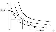
In order to understand the choice exercised by a consumer across different periods of time we take consumption in one period as a composite commodity. Suppose there is one consumer, $N$ commodities, and two periods. Preferences are given by $U(x_1, x_2)$ where $x_t = (x_{t1},\dots,x_{tN})$ . Income in period $t$ is $Y_{t}$ . Savings in period 1 is $S_{1}$ , spending in period $t$ is $C_{t}$ , and $r$ is the interest rate. If the person is unable to borrow against future income in the first period, then he is subject to separate budget constraints in each period:

C_{1}+S_{1}\leq Y_{1},

(1)

C_{2}\leq Y_{2}+S_{1}(1+r).

(2)

On the other hand, if such borrowing is possible then the person is subject to a single intertemporal budget constraint:

C_{1}+{\frac {C_{2}}{1+r}}=Y_{1}+{\frac {Y_{2}}{1+r}}.

(3)

The left hand side shows the present value of expenditure and right hand side depicts the present value of income. Multiplying the equation by $(1+r)$ would give us the corresponding future values.

Now the consumer has to choose a $C_{1}$ and $C_{2}$ so as to

Maximize

U(C_1,C_2)

subject to

C_{1}+C_{2}/(1+r)=Y_{1}+Y_{2}/(1+r).

If the consumer is a net saver, an increase in interest rate will have an ambiguous effect on the current consumption.

If the consumer is a net borrower, an increase in interest rate will reduce his current consumption.

A consumer may be a net saver or a net borrower. If he's initially at a level of consumption where he's neither a net borrower nor a net saver, an increase in income may make him a net saver or a net borrower depending on his preferences. An increase in current income or future income will increase current and future consumption(consumption smoothing motives).

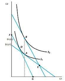
Now, let us consider a scenario where the interest rates are increased. If the consumer is a net saver, he will save more in the current period due to the substitution effect and consume more in the current period due to the income effect. The net effect thus becomes ambiguous. If the consumer is a net borrower, however, he will tend to consume less in the current period due to the substitution effect and income effect thereby reducing his overall current consumption.^[3]

Modigliani's life cycle income hypothesis

The life cycle hypothesis is based on the following model:

\max U_{t}=\sum _{t}U(C_{t})(1+\delta )^{{-t}}

subject to

\sum _{t}C_{t}(1+r)^{{-t}}=\sum _{t}Y_{t}(1+r)^{{-t}}+W_{0},

where

U(C_t) is satisfaction received from consumption in time period t,

C_t is the level of consumption at time t,

Y_t is income at time t,

δ is the rate of time preference ( a measure of individual preference between present and future activity),

W₀ is the initial level of income producing assets.

Life Cycle Hypothesis

Typically, a person's MPC (marginal propensity to consume) is relatively high during young adulthood, decreases during the middle-age years, and increases when the person is near or in retirement. The Life Cycle Hypothesis(LCH) model defines individual behavior as an attempt to smooth out consumption patterns over one's lifetime somewhat independent of current levels of income. This model states that early in one's life consumption expenditure may very well exceed income as the individual may be making major purchases related to buying a new home, starting a family, and beginning a career. At this stage in life the individual will borrow from the future to support these expenditure needs. In mid-life however, these expenditure patterns begin to level off and are supported or perhaps exceeded by increases in income. At this stage the individual repays any past borrowings and begins to save for her or his retirement. Upon retirement, consumption expenditure may begin to decline however income usually declines dramatically. In this stage of life, the individual dis-saves or lives off past savings until death.^[4]^[5]

Friedman's permanent income hypothesis

After the Second World War, it was noticed that a model in which current consumption was just a function of current income clearly was too simplistic. It could not explain the fact that the long-run average propensity to consume seemed to be roughly constant despite the marginal propensity to consume being much lower. Thus Milton Friedman's permanent income hypothesis is one of the models which seeks to explain this apparent contradiction.

According to the permanent income hypothesis, permanent consumption, C_P, is proportional to permanent income, Y_P. Permanent income is a subjective notion of likely average future income. Permanent consumption is a similar notion of consumption.

Actual consumption, C, and actual income, Y, consist of these permanent components plus unanticipated transitory components, C_T and Y_T, respectively:^[6]

C^P_t =β₂Y^P_t

C_t = C^P_t + C^T_t

Y_t = Y^P_t + Y^T_t

Labor supply

The choice of an individual as to how much labor to currently supply involves a trade-off between current labor and leisure. The amount of labor currently supplied influences not only current consumption opportunities but also future ones, and in particular influences the future choice of when to retire and supply no more labor. Thus the current labor supply choice is an intertemporal choice.

Fixed investment

Fixed investment is the purchasing by firms of newly produced machinery, factories, and the like. The reason for such purchases is to increase the amount of output that can potentially be produced at various times in the future, so this is an intertemporal choice.

Hyperbolic discounting

The article so far has considered cases where individuals make intertemporal choices by considering the present discounted value of their consumption and income. Every period in the future is exponentially discounted with the same interest rate. A different class of economists, however, argue that individuals are often affected by what is called the temporal myopia. The consumer's typical response to uncertainty in this case is to sharply reduce the importance of the future of their decision making.This effect is called hyperbolic discounting. In the common tongue it reflects the sentiment “Eat, drink and be merry, for tomorrow we may die.”^[7]

Mathematically, it may be represented as follows:

f_H(D)=\frac{1}{1+kD}\,

where

f(D) is the discount factor,

D is the delay in the reward, and

k is a parameter governing the degree of discounting.^[8]

When choosing between $100 or $110 a day later, individuals may impatiently choose the immediate $100 rather than wait for tomorrow for an extra $10. Yet, when choosing between $100 in a month or $110 in a month and a day, many of these people will reverse their preferences and now patiently choose to wait the additional day for the extra $10.^[9]

References

↑ Berns, Gregory S.; Laibson, David; Loewenstein, George (2007). "Intertemporal choice – Toward an Integrative Framework" (PDF). Trends in Cognitive Sciences. 11 (11): 482. doi:10.1016/j.tics.2007.08.011. PMID 17980645. Archived from the original on 2016-05-30.
↑ Thaler, Richard H. (1997). "Irving Fisher: Modern Behavioral Economist" (PDF). The American Economic Review. 87 (2): 439–441. JSTOR 2950963. Archived from the original on 2016-03-04.
↑ Varian, Hal (2006). Intermediate Micro Economics.
↑ Barro, Robert J. (1998). Macroeconomics (5th ed.). Cambridge, Mass.: MIT Press. ISBN 9780262024365.
↑ Mankiw, N. Gregory (2008). Principles of Macroeconomics (5th ed.). Cengage Learning. ISBN 9780324589993.
↑ "Adaptive expectations: Friedman's permanent income hypothesis".
↑ Bellows, Alan. "Hyperbolic Discounting".
↑ Hyperbolic discounting
↑ P. Redden, Joseph. "Hyperbolic Discounting".

This article is issued from Wikipedia. The text is licensed under Creative Commons - Attribution - Sharealike. Additional terms may apply for the media files.

[Berns2007-1] Berns, Gregory S.; Laibson, David; Loewenstein, George (2007). "Intertemporal choice – Toward an Integrative Framework" (PDF). Trends in Cognitive Sciences. 11 (11): 482. doi:10.1016/j.tics.2007.08.011. PMID 17980645. Archived from the original on 2016-05-30.

[Thaler1997-2] Thaler, Richard H. (1997). "Irving Fisher: Modern Behavioral Economist" (PDF). The American Economic Review. 87 (2): 439–441. JSTOR 2950963. Archived from the original on 2016-03-04.

[3] Varian, Hal (2006). Intermediate Micro Economics.

[4] Barro, Robert J. (1998). Macroeconomics (5th ed.). Cambridge, Mass.: MIT Press. ISBN 9780262024365.

[Mankiw2008-5] Mankiw, N. Gregory (2008). Principles of Macroeconomics (5th ed.). Cengage Learning. ISBN 9780324589993.

[6] "Adaptive expectations: Friedman's permanent income hypothesis".

[7] Bellows, Alan. "Hyperbolic Discounting".

[8] Hyperbolic discounting

[9] P. Redden, Joseph. "Hyperbolic Discounting".