Gravity anomaly
A gravity anomaly is the difference between the observed acceleration of free fall, or gravity, on a planet's surface, and the corresponding value predicted from a model of the planet's gravity field. Typically the model is based on simplifying assumptions, such as that, under its self-gravitation and rotational motion, the planet assumes the figure of an ellipsoid of revolution. Gravity on the surface of this reference ellipsoid is then given by a simple formula which only contains the latitude, and subtraction from observed gravity in the same location will yield the gravity anomaly.
Anomaly values are typically much smaller than the values of gravity itself, as the bulk contributions of the total mass of the planet, of its rotation and of its associated flattening, have been subtracted. As such, gravity anomalies describe the local variations of the gravity field around the model field. A location with a positive anomaly exhibits more gravity than predicted by the model—suggesting the presence of a sub-surface positive mass anomaly, while a negative anomaly exhibits a lower value than predicted—suggestive of a sub-surface mass deficit. These anomalies are thus of substantial geophysical and geological interest.
When gravity measurements have been made on the topography above sea level, a careful reduction process, also involving the effect of local topographic masses, must be carried out to obtain geophysically useful gravity anomalies, of which there are several different types. Cleanly extracting the response to the local sub-surface geology is the typical goal of applied geophysics.
Causes
Lateral variations in gravity anomalies are related to anomalous density distributions within the Earth. Gravity measures help us to understand the internal structure of the planet. Synthetic calculations show that the gravity anomaly signature of a thickened crust (for example, in orogenic belts produced by continental collision) is negative and larger in absolute value, relative to a case where thickening affects the entire lithosphere.
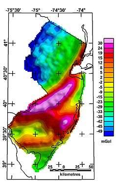
The Bouguer anomalies usually are negative in the mountains because they involve reducing out the attraction of the mountain mass, by about 100 milligals per kilometre of mountain height. In large mountain areas, they are even more negative than this because of isostasy: the rock density of the mountain roots is lower, compared with the surrounding earth's mantle, causing a further gravity deficit. Typical anomalies in the Central Alps are −150 milligals (−1.5 mm/s²). Rather local anomalies are used in applied geophysics: if they are positive, this may indicate metallic ores. At scales between entire mountain ranges and ore bodies, Bouguer anomalies may indicate rock types. For example, the northeast-southwest trending high across central New Jersey (see figure in the following section) represents a graben of Triassic age largely filled with dense basalts. Salt domes are typically expressed in gravity maps as lows, because salt has a low density compared to the rocks the dome intrudes. Anomalies can help to distinguish sedimentary basins whose fill differs in density from that of the surrounding region; see Gravity Anomalies of Britain and Ireland for example.
Geodesy and geophysics
In geodesy and geophysics, the usual theoretical model is the gravity on the surface of a reference ellipsoid such as WGS84.
To understand the nature of the gravity anomaly due to the subsurface, a number of corrections must be made to the measured gravity value:
- The theoretical gravity (smoothed normal gravity) should be removed in order to leave only local effects.
- The elevation of the point where each gravity measurement was taken must be reduced to a reference datum to compare the whole profile. This is called the Free-air Correction, and when combined with the removal of theoretical gravity leaves the free-air anomaly.
- the normal gradient of gravity (rate of change of gravity by change of elevation), as in free air, usually 0.3086 milligals per meter, or the Bouguer gradient of 0.1967 mGal/m (19.67 µm/(s²·m) which considers the mean rock density (2.67 g/cm³) beneath the point; this value is found by subtracting the gravity due to the Bouguer plate, which is 0.1119 mGal/m (11.19 µm/(s²·m)) for this density. Simply, we have to correct for the effects of any material between the point where gravimetry was done and the geoid. To do this we model the material in between as being made up of an infinite number of slabs of thickness t. These slabs have no lateral variation in density, but each slab may have a different density than the one above or below it. This is called the Bouguer correction.
- and (in special cases) a digital terrain model (DTM). A terrain correction, computed from a model structure, accounts for the effects of rapid lateral change in density, e.g. edge of plateau, cliffs, steep mountains, etc.
For these reductions, different methods are used:
- The gravity changes as we move away from the surface of the Earth. For this reason, we must compensate with the free-air anomaly (or Faye's anomaly): application of the normal gradient 0.3086 mGal/m, but no terrain model. This anomaly means a downward shift of the point, together with the whole shape of the terrain. This simple method is ideal for many geodetic applications.
- simple Bouguer anomaly: downward reduction just by the Bouguer gradient (0.1967). This anomaly handles the point as if it is located on a flat plain.
- refined (or complete) Bouguer anomaly (usual abbreviation ΔgB): the DTM is considered as accurate as possible, using a standard density of 2.67 g/cm³ (granite, limestone). Bouguer anomalies are ideal for geophysics because they show the effects of different rock densities in the subsurface.
- The difference between the two - the differential gravitational effect of the unevenness of the terrain - is called the terrain effect. It is always negative (up to 100 milligals).
- The difference between Faye anomaly and ΔgB is called Bouguer reduction (attraction of the terrain).
- special methods like that of Poincaré-Prey, using an interior gravity gradient of about 0.0848 milligal per meter (848 nm/(s²·m) or 11 h−2). These methods are valid for the gravity within boreholes or for special geoid computations.
Satellite measurements
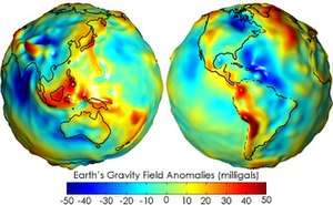
Large-scale gravity anomalies can be detected from space, as a by-product of satellite gravity missions, e.g., GOCE. These satellite missions aim at the recovery of a detailed gravity field model of the Earth, typically presented in the form of a spherical-harmonic expansion of the Earth's gravitational potential, but alternative presentations, such as maps of geoid undulations or gravity anomalies, are also produced.
The Gravity Recovery and Climate Experiment (GRACE) consists of two satellites that can detect gravitational changes across the Earth. Also these changes can be presented as gravity anomaly temporal variations.
References
Further reading
- Heiskanen, Weikko Aleksanteri; Moritz, Helmut (1967). Physical Geodesy. W.H. Freeman.