Duffing equation

The Duffing equation (or Duffing oscillator), named after Georg Duffing (1861–1944), is a non-linear second-order differential equation used to model certain damped and driven oscillators. The equation is given by

{\ddot {x}}+\delta {\dot {x}}+\alpha x+\beta x^{3}=\gamma \cos(\omega t)\,

A Poincaré section of the forced Duffing equation suggesting chaotic behaviour

(\alpha =1,

\beta =5,

\delta =0.02,

\gamma =8

and

\omega =0.5)

.

where the (unknown) function $x=x(t)$ is the displacement at time $t,$ ${\dot {x}}$ is the first derivative of $x$ with respect to time, i.e. velocity, and ${\ddot {x}}$ is the second time-derivative of $x,$ i.e. acceleration. The numbers $\delta ,$ $\alpha ,$ $\beta ,$ $\gamma$ and $\omega$ are given constants.

The equation describes the motion of a damped oscillator with a more complex potential than in simple harmonic motion (which corresponds to the case $\beta =\delta =0$ ); in physical terms, it models, for example, an elastic pendulum whose spring's stiffness does not exactly obey Hooke's law.

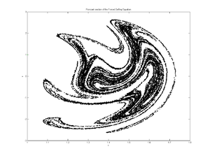
The Duffing equation is an example of a dynamical system that exhibits chaotic behavior. Moreover, the Duffing system presents in the frequency response the jump resonance phenomenon that is a sort of frequency hysteresis behaviour.

Parameters

The parameters in the above equation are:

$\delta$ controls the amount of damping,
$\alpha$ controls the linear stiffness,
$\beta$ controls the amount of non-linearity in the restoring force; if $\beta =0,$ the Duffing equation describes a damped and driven simple harmonic oscillator,
$\gamma$ is the amplitude of the periodic driving force; if $\gamma =0$ the system is without a driving force, and
$\omega$ is the angular frequency of the periodic driving force.

The Duffing equation can be seen as describing the oscillations of a mass attached to a nonlinear spring and a linear damper. The restoring force provided by the nonlinear spring is then $\alpha x+\beta x^{3}.$

When $\alpha >0$ and $\beta >0$ the spring is called a hardening spring. Conversely, for $\beta <0$ it is a softening spring (still with $\alpha >0$ ). Consequently, the adjectives hardening and softening are used with respect to the Duffing equation in general, dependent on the values of $\beta$ (and $\alpha$ ).[1]

The number of parameters in the Duffing equation can be reduced by two through scaling, e.g. the excursion $x$ and time $t$ can be scaled as:[2] $\tau =t{\sqrt {\alpha }}$ and $y=x\alpha /\gamma ,$ assuming $\alpha$ is positive (other scalings are possible for different ranges of the parameters, or for different emphasis in the problem studied). Then:[3]

{\ddot {y}}+2\eta \,{\dot {y}}+y+\varepsilon \,y^{3}=\cos(\sigma \tau ),

where

\eta ={\frac {\delta }{2{\sqrt {\alpha }}}},

\varepsilon ={\frac {\beta \gamma ^{2}}{\alpha ^{3}}}.

and

\sigma ={\frac {\omega }{\sqrt {\alpha }}}.

The dots denote differentiation of $y(\tau )$ with respect to $\tau .$ This shows that the solutions to the forced and damped Duffing equation can be described in terms of the three parameters ( $\varepsilon ,$ $\eta$ and $\sigma$ ) and two initial conditions (i.e. for $y(t_{0})$ and ${\dot {y}}(t_{0})$ ).

Methods of solution

In general, the Duffing equation does not admit an exact symbolic solution. However, many approximate methods work well:

Expansion in a Fourier series may provide an equation of motion to arbitrary precision.
The $x^{3}$ term, also called the Duffing term, can be approximated as small and the system treated as a perturbed simple harmonic oscillator.
The Frobenius method yields a complex but workable solution.
Any of the various numeric methods such as Euler's method and Runge-Kutta can be used.
The homotopy analysis method (HAM) has also been reported for obtaining approximate solutions of the Duffing equation, also for strong nonlinearity.[4][5]

In the special case of the undamped ( $\delta =0$ ) and undriven ( $\gamma =0$ ) Duffing equation, an exact solution can be obtained using Jacobi's elliptic functions.[6]

Boundedness of the solution for the unforced oscillator

Undamped oscillator

Multiplication of the undamped and unforced Duffing equation, $\gamma =\delta =0,$ with ${\dot {x}}$ gives:[7]

{\begin{aligned}&{\dot {x}}\left({\ddot {x}}+\alpha x+\beta x^{3}\right)=0\\&\Rightarrow {\frac {\mathrm {d} }{\mathrm {d} t}}\left[{\tfrac {1}{2}}\left({\dot {x}}\right)^{2}+{\tfrac {1}{2}}\alpha x^{2}+{\tfrac {1}{4}}\beta x^{4}\right]=0\\&\Rightarrow {\tfrac {1}{2}}\left({\dot {x}}\right)^{2}+{\tfrac {1}{2}}\alpha x^{2}+{\tfrac {1}{4}}\beta x^{4}=H,\end{aligned}}

with H a constant. The value of H is determined by the initial conditions $x(0)$ and ${\dot {x}}(0).$

The substitution $y={\dot {x}}$ in H shows that the system is Hamiltonian:

{\dot {x}}=+{\frac {\partial H}{\partial y}},

{\dot {y}}=-{\frac {\partial H}{\partial x}}

with

\quad H={\tfrac {1}{2}}y^{2}+{\tfrac {1}{2}}\alpha x^{2}+{\tfrac {1}{4}}\beta x^{4}.

When both $\alpha$ and $\beta$ are positive, the solution is bounded:[7]

|x|\leq {\sqrt {2H/\alpha }}

and

|{\dot {x}}|\leq {\sqrt {2H}},

with the Hamiltonian H being positive.

Damped oscillator

Similarly, for the damped oscillator,[8]

{\begin{aligned}&{\dot {x}}\left({\ddot {x}}+\delta {\dot {x}}+\alpha x+\beta x^{3}\right)=0\\&\Rightarrow {\frac {\mathrm {d} }{\mathrm {d} t}}\left[{\tfrac {1}{2}}\left({\dot {x}}\right)^{2}+{\tfrac {1}{2}}\alpha x^{2}+{\tfrac {1}{4}}\beta x^{4}\right]=-\delta \,\left({\dot {x}}\right)^{2}\\&\Rightarrow {\frac {\mathrm {d} H}{\mathrm {d} t}}=-\delta \,\left({\dot {x}}\right)^{2}\leq 0,\end{aligned}}

since $\delta \geq 0$ for damping. Without forcing the damped Duffing oscillator will end up at (one of) its stable equilibrium point(s). The equilibrium points, stable and unstable, are at $\alpha x+\beta x^{3}=0.$ If $\alpha >0$ the stable equilibrium is at $x=0.$ If $\alpha <0$ and $\beta >0$ the stable equilibria are at $x=+{\sqrt {-\alpha /\beta }}$ and $x=-{\sqrt {-\alpha /\beta }}.$

Frequency response

Frequency response

z/\gamma

as a function of

\omega /{\sqrt {\alpha }}

for the Duffing equation, with

\alpha =\gamma =1

and damping

\delta =0.1.

The dashed parts of the frequency response are unstable.[3]

The forced Duffing oscillator with cubic nonlinearity is described by the following ordinary differential equation:

{\ddot {x}}+\delta {\dot {x}}+\alpha x+\beta x^{3}=\gamma \cos(\omega t).

The frequency response of this oscillator describes the amplitude $z$ of steady state response of the equation (i.e. $x(t)$ ) at a given frequency of excitation $\omega .$ For a linear oscillator with $\beta =0,$ the frequency response is also linear. However, for a nonzero cubic coefficient, the frequency response becomes nonlinear. Depending on the type of nonlinearity, the Duffing oscillator can show hardening, softening or mixed hardening–softening frequency response. Anyway, using the homotopy analysis method or harmonic balance, one can derive a frequency response equation in the following form:[9][5]

\left[\left(\omega ^{2}-\alpha -{\frac {3}{4}}\beta z^{2}\right)^{2}+\left(\delta \omega \right)^{2}\right]\,z^{2}=\gamma ^{2}.

For the parameters of the Duffing equation, the above algebraic equation gives the steady state oscillation amplitude $z$ at a given excitation frequency.

Derivation of the frequency response

Using the method of harmonic balance, an approximate solution to the Duffing equation is sought of the form:[9]

x=a\,\cos(\omega t)+b\,\sin(\omega t)=z\,\cos(\omega t-\phi ),

with

z^{2}=a^{2}+b^{2}

and

\tan \phi ={\frac {b}{a}}.

Application in the Duffing equation leads to:

{\begin{aligned}&\left(-\omega ^{2}\,a+\omega \,\delta \,b+\alpha \,a+{\tfrac {3}{4}}\,\beta \,a^{3}+{\tfrac {3}{4}}\,\beta \,a\,b^{2}-\gamma \right)\,\cos \left(\omega \,t\right)\\&+\left(-\omega ^{2}\,b-\omega \,\delta \,a+{\tfrac {3}{4}}\,\beta \,b^{3}+\alpha \,b+{\tfrac {3}{4}}\,\beta \,a^{2}\,b\right)\,\sin \left(\omega \,t\right)\\&+\left({\tfrac {1}{4}}\,\beta \,a^{3}-{\tfrac {3}{4}}\,\beta \,a\,b^{2}\right)\,\cos \left(3\,\omega \,t\right)+\left({\tfrac {3}{4}}\,\beta \,a^{2}\,b-{\tfrac {1}{4}}\,\beta \,b^{3}\right)\,\sin \left(3\,\omega \,t\right)=0.\end{aligned}}

Neglecting the superharmonics at $3\omega ,$ the two terms preceding $\cos(\omega t)$ and $\sin(\omega t)$ have to be zero. As a result,

{\begin{aligned}&-\omega ^{2}\,a+\omega \,\delta \,b+\alpha \,a+{\tfrac {3}{4}}\,\beta \,a^{3}+{\tfrac {3}{4}}\,\beta \,a\,b^{2}=\gamma \qquad {\text{and}}\\&-\omega ^{2}\,b-\omega \,\delta \,a+{\tfrac {3}{4}}\,\beta \,b^{3}+\alpha \,b+{\tfrac {3}{4}}\,\beta \,a^{2}\,b=0.\end{aligned}}

Squaring both equations and adding leads to the amplitude frequency response:

\left[\left(\omega ^{2}-\alpha -{\frac {3}{4}}\beta z^{2}\right)^{2}+\left(\delta \omega \right)^{2}\right]\,z^{2}=\gamma ^{2},

as stated above.

Jumps

Jumps in the frequency response. The parameters are:

\alpha =\gamma =1,

,

\beta =0.04

and

\delta =0.1.

[9]

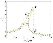
For certain ranges of the parameters in the Duffing equation, the frequency response may no longer be a single-valued function of forcing frequency $\omega .$ For a hardening spring oscillator ( $\alpha >0$ and large enough positive $\beta >\beta _{c+}>0$ ) the frequency response overhangs to the high-frequency side, and to the low-frequency side for the softening spring oscillator ( $\alpha >0$ and $\beta <\beta _{c-}<0$ ). The lower overhanging side is unstable – i.e. the dashed-line parts in the figures of the frequency response – and cannot be realized for a sustained time. Consequently, the jump phenomenon shows up:

when the angular frequency $\omega$ is slowly increased (with other parameters fixed), the response amplitude $z$ drops at A suddenly to B,
if the frequency $\omega$ is slowly decreased, then at C the amplitude jumps up to D, thereafter following the upper branch of the frequency response.

The jumps A–B and C–D do not coincide, so the system shows hysteresis depending on the frequency sweep direction.[9]

Examples

Time traces and phase portraits

period-1 oscillation at

\gamma =0.20

period-2 oscillation at

\gamma =0.28

period-4 oscillation at

\gamma =0.29

period-5 oscillation at

\gamma =0.37

chaos at

\gamma =0.50

period-2 oscillation at

\gamma =0.65

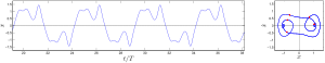
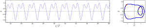
Some typical examples of the time series and phase portraits of the Duffing equation, showing the appearance of subharmonics through period-doubling bifurcation – as well chaotic behavior – are shown in the figures below. The forcing amplitude increases from $\gamma =0.20$ to $\gamma =0.65.$ The other parameters have the values: $\alpha =-1,$ $\beta =+1,$ $\delta =0.3$ and $\omega =1.2.$ The initial conditions are $x(0)=1$ and ${\dot {x}}(0)=0.$ The red dots in the phase portraits are at times $t$ which are an integer multiple of the period $T=2\pi /\omega .$ [10]

References

Inline

Thompson, J.M.T.; Stewart, H.B. (2002). Nonlinear Dynamics and Chaos. John Wiley & Sons. p. 66. ISBN 9780471876847.
Lifshitz, R.; Cross, M.C. (2008). "Nonlinear mechanics of nanomechanical and micromechanical resonators". In Schuster, H.G. (ed.). Reviews of Nonlinear Dynamics and Complexity. Wiley. pp. 8–9. ISBN 9783527407293. LCCN 2008459659.
Brennan, M.J.; Kovacic, I.; Carrella, A.; Waters, T.P. (2008). "On the jump-up and jump-down frequencies of the Duffing oscillator". Journal of Sound and Vibration. 318 (4–5): 1250–1261. doi:10.1016/j.jsv.2008.04.032.
Kovacic & Brennan (2011, pp. 123–127)
Tajaddodianfar, F.; Yazdi, M.R.H.; Pishkenari, H.N. (2016). "Nonlinear dynamics of MEMS/NEMS resonators: analytical solution by the homotopy analysis method". Microsystem Technologies. doi:10.1007/s00542-016-2947-7.
Rand, R.H. (2012), Lecture notes on nonlinear vibrations (PDF), 53, Cornell University, pp. 13–17
Bender & Orszag (1999, p. 546)
Takashi Kanamaru (ed.). "Duffing oscillator". Scholarpedia.
Jordan & Smith (2007, pp. 223–233)
Based on the examples shown in Jordan & Smith (2007, pp. 453–462)

Historical

Duffing, G. (1918), Erzwungene Schwingungen bei veränderlicher Eigenfrequenz und ihre technische Bedeutung [Forced oscillations with variable natural frequency and their technical relevance] (in German), Heft 41/42, Braunschweig: Vieweg, vi+134 pp., OCLC 12003652

Other

Addison, P.S. (1997), Fractals and Chaos: An illustrated course, CRC Press, pp. 147–148, ISBN 9780849384431
Bender, C.M.; Orszag, S.A. (1999), Advanced Mathematical Methods for Scientists and Engineers I: Asymptotic Methods and Perturbation Theory, Springer, pp. 545–551, ISBN 9780387989310
Jordan, D.W.; Smith, P. (2007), Nonlinear ordinary differential equations – An introduction for scientists and engineers (4th ed.), Oxford University Press, ISBN 978-0-19-920824-1
Kovacic, I.; Brennan, M.J., eds. (2011), The Duffing Equation: Nonlinear Oscillators and their Behaviour, Wiley, 392 pp., ISBN 978-0-470-71549-9

External links

This article is issued from Wikipedia. The text is licensed under Creative Commons - Attribution - Sharealike. Additional terms may apply for the media files.

[1] Thompson, J.M.T.; Stewart, H.B. (2002). Nonlinear Dynamics and Chaos. John Wiley & Sons. p. 66. ISBN 9780471876847.

[2] Lifshitz, R.; Cross, M.C. (2008). "Nonlinear mechanics of nanomechanical and micromechanical resonators". In Schuster, H.G. (ed.). Reviews of Nonlinear Dynamics and Complexity. Wiley. pp. 8–9. ISBN 9783527407293. LCCN 2008459659.

[BKCW2008-3] Brennan, M.J.; Kovacic, I.; Carrella, A.; Waters, T.P. (2008). "On the jump-up and jump-down frequencies of the Duffing oscillator". Journal of Sound and Vibration. 318 (4–5): 1250–1261. doi:10.1016/j.jsv.2008.04.032.

[4] Kovacic & Brennan (2011, pp. 123–127)

[ReferenceA-5] Tajaddodianfar, F.; Yazdi, M.R.H.; Pishkenari, H.N. (2016). "Nonlinear dynamics of MEMS/NEMS resonators: analytical solution by the homotopy analysis method". Microsystem Technologies. doi:10.1007/s00542-016-2947-7.

[6] Rand, R.H. (2012), Lecture notes on nonlinear vibrations (PDF), 53, Cornell University, pp. 13–17

[BO99-7] Bender & Orszag (1999, p. 546)

[8] Takashi Kanamaru (ed.). "Duffing oscillator". Scholarpedia.

[JordanSmith-9] Jordan & Smith (2007, pp. 223–233)

[10] Based on the examples shown in Jordan & Smith (2007, pp. 453–462)

Chaos theory
Chaos theory	Anosov diffeomorphism Bifurcation theory Butterfly effect Chaos theory in organizational development Complexity Control of chaos Dynamical system Edge of chaos Fractal Predictability Quantum chaos Santa Fe Institute Synchronization of chaos Unintended consequences
Chaotic maps (list)	Arnold tongue Arnold's cat map Baker's map Complex quadratic map Complex squaring map Coupled map lattice Double pendulum Double scroll attractor Duffing equation Duffing map Dyadic transformation Dynamical billiards outer Elastic pendulum Exponential map Gauss map Gingerbreadman map Hénon map Horseshoe map Ikeda map Interval exchange map Kaplan–Yorke map Logistic map Lorenz system Multiscroll attractor Rabinovich–Fabrikant equations Rössler attractor Standard map Swinging Atwood's machine Tent map Three-body problem Tinkerbell map Van der Pol oscillator Zaslavskii map
Chaos systems	Bouncing ball dynamics Chua's circuit Economic bubble FPUT problem Tilt-A-Whirl
Chaos theorists	Michael Berry Mary Cartwright Leon O. Chua Mitchell Feigenbaum Celso Grebogi Martin Gutzwiller Brosl Hasslacher Michel Hénon Svetlana Jitomirskaya Bryna Kra Edward Norton Lorenz Aleksandr Lyapunov Benoît Mandelbrot Hee Oh Edward Ott Henri Poincaré Mary Rees Otto Rössler David Ruelle Caroline Series Oleksandr Mykolayovych Sharkovsky Nina Snaith Floris Takens Audrey Terras Mary Tsingou Amie Wilkinson James A. Yorke Lai-Sang Young