Fourier series

If ${\displaystyle s(x)}$ is a complex-valued function of a real variable ${\displaystyle x,}$ both components (real and imaginary part) are real-valued functions that can be represented by a Fourier series. The two sets of coefficients and the partial sum are given by:

${\displaystyle c_{_{Rn}}={\frac {1}{P}}\int _{P}\operatorname {Re} \{s(x)\}\cdot e^{-i{\tfrac {2\pi nx}{P}}}\ dx}$     and     ${\displaystyle c_{_{In}}={\frac {1}{P}}\int _{P}\operatorname {Im} \{s(x)\}\cdot e^{-i{\tfrac {2\pi nx}{P}}}\ dx}$

${\displaystyle s_{N}(x)=\sum _{n=-N}^{N}c_{_{Rn}}\cdot e^{i{\tfrac {2\pi nx}{P}}}+i\cdot \sum _{n=-N}^{N}c_{_{In}}\cdot e^{i{\tfrac {2\pi nx}{P}}}=\sum _{n=-N}^{N}\left(c_{_{Rn}}+i\cdot c_{_{In}}\right)\cdot e^{i{\tfrac {2\pi nx}{P}}}.}$

Defining ${\displaystyle c_{n}\triangleq c_{_{Rn}}+i\cdot c_{_{In}}}$ yields:

${\displaystyle s_{N}(x)=\sum _{n=-N}^{N}c_{n}\cdot e^{i{\tfrac {2\pi nx}{P}}}.}$

(Eq.5)

This is identical to Eq.4 except ${\displaystyle c_{n}}$ and ${\displaystyle c_{-n}}$ are no longer complex conjugates. The formula for ${\displaystyle c_{n}}$ is also unchanged:

${\displaystyle {\begin{aligned}c_{n}&={\frac {1}{P}}\int _{P}\operatorname {Re} \{s(x)\}\cdot e^{-i{\tfrac {2\pi nx}{P}}}\ dx+i\cdot {\frac {1}{P}}\int _{P}\operatorname {Im} \{s(x)\}\cdot e^{-i{\tfrac {2\pi nx}{P}}}\ dx\\[4pt]&={\frac {1}{P}}\int _{P}\left(\operatorname {Re} \{s(x)\}+i\cdot \operatorname {Im} \{s(x)\}\right)\cdot e^{-i{\tfrac {2\pi nx}{P}}}\ dx\ =\ {\frac {1}{P}}\int _{P}s(x)\cdot e^{-i{\tfrac {2\pi nx}{P}}}\ dx.\end{aligned}}}$

The notation ${\displaystyle c_{n}}$ is inadequate for discussing the Fourier coefficients of several different functions. Therefore, it is customarily replaced by a modified form of the function (${\displaystyle s}$, in this case), such as ${\displaystyle {\hat {s}}(n)}$ or ${\displaystyle S[n]}$, and functional notation often replaces subscripting:

${\displaystyle {\begin{aligned}s_{\infty }(x)&=\sum _{n=-\infty }^{\infty }{\hat {s}}(n)\cdot e^{i\,2\pi nx/P}\\[6pt]&=\sum _{n=-\infty }^{\infty }S[n]\cdot e^{j\,2\pi nx/P}&&\scriptstyle {\mathsf {common\ engineering\ notation}}\end{aligned}}}$

In engineering, particularly when the variable ${\displaystyle x}$ represents time, the coefficient sequence is called a frequency domain representation. Square brackets are often used to emphasize that the domain of this function is a discrete set of frequencies.

Another commonly used frequency domain representation uses the Fourier series coefficients to modulate a Dirac comb:

${\displaystyle S(f)\ \triangleq \ \sum _{n=-\infty }^{\infty }S[n]\cdot \delta \left(f-{\frac {n}{P}}\right),}$

where ${\displaystyle f}$ represents a continuous frequency domain. When variable ${\displaystyle x}$ has units of seconds, ${\displaystyle f}$ has units of hertz. The "teeth" of the comb are spaced at multiples (i.e. harmonics) of ${\displaystyle 1/P}$, which is called the fundamental frequency.  ${\displaystyle s_{\infty }(x)}$  can be recovered from this representation by an inverse Fourier transform:

${\displaystyle {\begin{aligned}{\mathcal {F}}^{-1}\{S(f)\}&=\int _{-\infty }^{\infty }\left(\sum _{n=-\infty }^{\infty }S[n]\cdot \delta \left(f-{\frac {n}{P}}\right)\right)e^{i2\pi fx}\,df,\\[6pt]&=\sum _{n=-\infty }^{\infty }S[n]\cdot \int _{-\infty }^{\infty }\delta \left(f-{\frac {n}{P}}\right)e^{i2\pi fx}\,df,\\[6pt]&=\sum _{n=-\infty }^{\infty }S[n]\cdot e^{i\,2\pi nx/P}\ \ \triangleq \ s_{\infty }(x).\end{aligned}}}$

The constructed function ${\displaystyle S(f)}$ is therefore commonly referred to as a Fourier transform, even though the Fourier integral of a periodic function is not convergent at the harmonic frequencies.[upper-alpha 2]

Plot of the sawtooth wave, a periodic continuation of the linear function ${\displaystyle s(x)=x/\pi }$ on the interval ${\displaystyle (-\pi ,\pi ]}$

Animated plot of the first five successive partial Fourier series

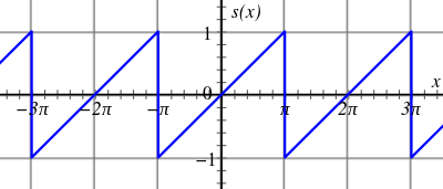
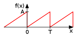
We now use the formula above to give a Fourier series expansion of a very simple function. Consider a sawtooth wave

${\displaystyle s(x)={\frac {x}{\pi }},\quad \mathrm {for} -\pi <x<\pi ,}$

${\displaystyle s(x+2\pi k)=s(x),\quad \mathrm {for} -\pi <x<\pi {\text{ and }}k\in \mathbb {Z} .}$

In this case, the Fourier coefficients are given by

${\displaystyle {\begin{aligned}a_{n}&={\frac {1}{\pi }}\int _{-\pi }^{\pi }s(x)\cos(nx)\,dx=0,\quad n\geq 0.\\[4pt]b_{n}&={\frac {1}{\pi }}\int _{-\pi }^{\pi }s(x)\sin(nx)\,dx\\[4pt]&=-{\frac {2}{\pi n}}\cos(n\pi )+{\frac {2}{\pi ^{2}n^{2}}}\sin(n\pi )\\[4pt]&={\frac {2\,(-1)^{n+1}}{\pi n}},\quad n\geq 1.\end{aligned}}}$

It can be proven that Fourier series converges to ${\displaystyle s(x)}$ at every point ${\displaystyle x}$ where ${\displaystyle s}$ is differentiable, and therefore:

${\displaystyle {\begin{aligned}s(x)&={\frac {a_{0}}{2}}+\sum _{n=1}^{\infty }\left[a_{n}\cos \left(nx\right)+b_{n}\sin \left(nx\right)\right]\\[4pt]&={\frac {2}{\pi }}\sum _{n=1}^{\infty }{\frac {(-1)^{n+1}}{n}}\sin(nx),\quad \mathrm {for} \quad x-\pi \notin 2\pi \mathbb {Z} .\end{aligned}}}$

(Eq.7)

When ${\displaystyle x=\pi }$, the Fourier series converges to 0, which is the half-sum of the left- and right-limit of s at ${\displaystyle x=\pi }$. This is a particular instance of the Dirichlet theorem for Fourier series.

Heat distribution in a metal plate, using Fourier's method

This example leads us to a solution to the Basel problem.

The Fourier series expansion of our function in Example 1 looks more complicated than the simple formula ${\displaystyle s(x)=x/\pi }$, so it is not immediately apparent why one would need the Fourier series. While there are many applications, Fourier's motivation was in solving the heat equation. For example, consider a metal plate in the shape of a square whose side measures ${\displaystyle \pi }$ meters, with coordinates ${\displaystyle (x,y)\in [0,\pi ]\times [0,\pi ]}$. If there is no heat source within the plate, and if three of the four sides are held at 0 degrees Celsius, while the fourth side, given by ${\displaystyle y=\pi }$, is maintained at the temperature gradient ${\displaystyle T(x,\pi )=x}$ degrees Celsius, for ${\displaystyle x}$ in ${\displaystyle (0,\pi )}$, then one can show that the stationary heat distribution (or the heat distribution after a long period of time has elapsed) is given by

${\displaystyle T(x,y)=2\sum _{n=1}^{\infty }{\frac {(-1)^{n+1}}{n}}\sin(nx){\sinh(ny) \over \sinh(n\pi )}.}$

Here, sinh is the hyperbolic sine function. This solution of the heat equation is obtained by multiplying each term of  Eq.7 by ${\displaystyle \sinh(ny)/\sinh(n\pi )}$. While our example function ${\displaystyle s(x)}$ seems to have a needlessly complicated Fourier series, the heat distribution ${\displaystyle T(x,y)}$ is nontrivial. The function ${\displaystyle T}$ cannot be written as a closed-form expression. This method of solving the heat problem was made possible by Fourier's work.

Another application of this Fourier series is to solve the Basel problem by using Parseval's theorem. The example generalizes and one may compute ζ(2n), for any positive integer n.

Since Fourier's time, many different approaches to defining and understanding the concept of Fourier series have been discovered, all of which are consistent with one another, but each of which emphasizes different aspects of the topic. Some of the more powerful and elegant approaches are based on mathematical ideas and tools that were not available at the time Fourier completed his original work. Fourier originally defined the Fourier series for real-valued functions of real arguments, and using the sine and cosine functions as the basis set for the decomposition.

Many other Fourier-related transforms have since been defined, extending the initial idea to other applications. This general area of inquiry is now sometimes called harmonic analysis. A Fourier series, however, can be used only for periodic functions, or for functions on a bounded (compact) interval.

We can also define the Fourier series for functions of two variables ${\displaystyle x}$ and ${\displaystyle y}$ in the square ${\displaystyle [-\pi ,\pi ]\times [-\pi ,\pi ]}$:

${\displaystyle {\begin{aligned}f(x,y)&=\sum _{j,k\,\in \,\mathbb {Z} {\text{ (integers)}}}c_{j,k}e^{ijx}e^{iky},\\[5pt]c_{j,k}&={1 \over 4\pi ^{2}}\int _{-\pi }^{\pi }\int _{-\pi }^{\pi }f(x,y)e^{-ijx}e^{-iky}\,dx\,dy.\end{aligned}}}$

Aside from being useful for solving partial differential equations such as the heat equation, one notable application of Fourier series on the square is in image compression. In particular, the jpeg image compression standard uses the two-dimensional discrete cosine transform, which is a Fourier transform using the cosine basis functions.

The three-dimensional Bravais lattice is defined as the set of vectors of the form:

${\displaystyle \mathbf {R} =n_{1}\mathbf {a} _{1}+n_{2}\mathbf {a} _{2}+n_{3}\mathbf {a} _{3}}$

where ${\displaystyle n_{i}}$ are integers and ${\displaystyle \mathbf {a} _{i}}$ are three linearly independent vectors. Assuming we have some function, ${\displaystyle f(\mathbf {r} )}$, such that it obeys the following condition for any Bravais lattice vector ${\displaystyle \mathbf {R} :f(\mathbf {r} )=f(\mathbf {R} +\mathbf {r} )}$, we could make a Fourier series of it. This kind of function can be, for example, the effective potential that one electron "feels" inside a periodic crystal. It is useful to make a Fourier series of the potential then when applying Bloch's theorem. First, we may write any arbitrary vector ${\displaystyle \mathbf {r} }$ in the coordinate-system of the lattice:

${\displaystyle \mathbf {r} =x_{1}{\frac {\mathbf {a} _{1}}{a_{1}}}+x_{2}{\frac {\mathbf {a} _{2}}{a_{2}}}+x_{3}{\frac {\mathbf {a} _{3}}{a_{3}}},}$

where ${\displaystyle a_{i}\triangleq |\mathbf {a} _{i}|.}$

Thus we can define a new function,

${\displaystyle g(x_{1},x_{2},x_{3})\triangleq f(\mathbf {r} )=f\left(x_{1}{\frac {\mathbf {a} _{1}}{a_{1}}}+x_{2}{\frac {\mathbf {a} _{2}}{a_{2}}}+x_{3}{\frac {\mathbf {a} _{3}}{a_{3}}}\right).}$

This new function, ${\displaystyle g(x_{1},x_{2},x_{3})}$, is now a function of three-variables, each of which has periodicity a₁, a₂, a₃ respectively:

${\displaystyle g(x_{1},x_{2},x_{3})=g(x_{1}+a_{1},x_{2},x_{3})=g(x_{1},x_{2}+a_{2},x_{3})=g(x_{1},x_{2},x_{3}+a_{3}).}$

If we write a series for g on the interval [0, a₁] for x₁, we can define the following:

${\displaystyle h^{\mathrm {one} }(m_{1},x_{2},x_{3})\triangleq {\frac {1}{a_{1}}}\int _{0}^{a_{1}}g(x_{1},x_{2},x_{3})\cdot e^{-i2\pi {\frac {m_{1}}{a_{1}}}x_{1}}\,dx_{1}}$

And then we can write:

${\displaystyle g(x_{1},x_{2},x_{3})=\sum _{m_{1}=-\infty }^{\infty }h^{\mathrm {one} }(m_{1},x_{2},x_{3})\cdot e^{i2\pi {\frac {m_{1}}{a_{1}}}x_{1}}}$

Further defining:

${\displaystyle {\begin{aligned}h^{\mathrm {two} }(m_{1},m_{2},x_{3})&\triangleq {\frac {1}{a_{2}}}\int _{0}^{a_{2}}h^{\mathrm {one} }(m_{1},x_{2},x_{3})\cdot e^{-i2\pi {\frac {m_{2}}{a_{2}}}x_{2}}\,dx_{2}\\[12pt]&={\frac {1}{a_{2}}}\int _{0}^{a_{2}}dx_{2}{\frac {1}{a_{1}}}\int _{0}^{a_{1}}dx_{1}g(x_{1},x_{2},x_{3})\cdot e^{-i2\pi \left({\frac {m_{1}}{a_{1}}}x_{1}+{\frac {m_{2}}{a_{2}}}x_{2}\right)}\end{aligned}}}$

We can write ${\displaystyle g}$ once again as:

${\displaystyle g(x_{1},x_{2},x_{3})=\sum _{m_{1}=-\infty }^{\infty }\sum _{m_{2}=-\infty }^{\infty }h^{\mathrm {two} }(m_{1},m_{2},x_{3})\cdot e^{i2\pi {\frac {m_{1}}{a_{1}}}x_{1}}\cdot e^{i2\pi {\frac {m_{2}}{a_{2}}}x_{2}}}$

Finally applying the same for the third coordinate, we define:

${\displaystyle {\begin{aligned}h^{\mathrm {three} }(m_{1},m_{2},m_{3})&\triangleq {\frac {1}{a_{3}}}\int _{0}^{a_{3}}h^{\mathrm {two} }(m_{1},m_{2},x_{3})\cdot e^{-i2\pi {\frac {m_{3}}{a_{3}}}x_{3}}\,dx_{3}\\[12pt]&={\frac {1}{a_{3}}}\int _{0}^{a_{3}}dx_{3}{\frac {1}{a_{2}}}\int _{0}^{a_{2}}dx_{2}{\frac {1}{a_{1}}}\int _{0}^{a_{1}}dx_{1}g(x_{1},x_{2},x_{3})\cdot e^{-i2\pi \left({\frac {m_{1}}{a_{1}}}x_{1}+{\frac {m_{2}}{a_{2}}}x_{2}+{\frac {m_{3}}{a_{3}}}x_{3}\right)}\end{aligned}}}$

We write ${\displaystyle g}$ as:

${\displaystyle g(x_{1},x_{2},x_{3})=\sum _{m_{1}=-\infty }^{\infty }\sum _{m_{2}=-\infty }^{\infty }\sum _{m_{3}=-\infty }^{\infty }h^{\mathrm {three} }(m_{1},m_{2},m_{3})\cdot e^{i2\pi {\frac {m_{1}}{a_{1}}}x_{1}}\cdot e^{i2\pi {\frac {m_{2}}{a_{2}}}x_{2}}\cdot e^{i2\pi {\frac {m_{3}}{a_{3}}}x_{3}}}$

Re-arranging:

${\displaystyle g(x_{1},x_{2},x_{3})=\sum _{m_{1},m_{2},m_{3}\in \mathbb {Z} }h^{\mathrm {three} }(m_{1},m_{2},m_{3})\cdot e^{i2\pi \left({\frac {m_{1}}{a_{1}}}x_{1}+{\frac {m_{2}}{a_{2}}}x_{2}+{\frac {m_{3}}{a_{3}}}x_{3}\right)}.}$

Now, every reciprocal lattice vector can be written as ${\displaystyle \mathbf {G} =\ell _{1}\mathbf {g} _{1}+\ell _{2}\mathbf {g} _{2}+\ell _{3}\mathbf {g} _{3}}$, where ${\displaystyle l_{i}}$ are integers and ${\displaystyle \mathbf {g} _{i}}$ are the reciprocal lattice vectors, we can use the fact that ${\displaystyle \mathbf {g_{i}} \cdot \mathbf {a_{j}} =2\pi \delta _{ij}}$ to calculate that for any arbitrary reciprocal lattice vector ${\displaystyle \mathbf {G} }$ and arbitrary vector in space ${\displaystyle \mathbf {r} }$, their scalar product is:

${\displaystyle \mathbf {G} \cdot \mathbf {r} =\left(\ell _{1}\mathbf {g} _{1}+\ell _{2}\mathbf {g} _{2}+\ell _{3}\mathbf {g} _{3}\right)\cdot \left(x_{1}{\frac {\mathbf {a} _{1}}{a_{1}}}+x_{2}{\frac {\mathbf {a} _{2}}{a_{2}}}+x_{3}{\frac {\mathbf {a} _{3}}{a_{3}}}\right)=2\pi \left(x_{1}{\frac {\ell _{1}}{a_{1}}}+x_{2}{\frac {\ell _{2}}{a_{2}}}+x_{3}{\frac {\ell _{3}}{a_{3}}}\right).}$

And so it is clear that in our expansion, the sum is actually over reciprocal lattice vectors:

${\displaystyle f(\mathbf {r} )=\sum _{\mathbf {G} }h(\mathbf {G} )\cdot e^{i\mathbf {G} \cdot \mathbf {r} },}$

where

${\displaystyle h(\mathbf {G} )={\frac {1}{a_{3}}}\int _{0}^{a_{3}}dx_{3}\,{\frac {1}{a_{2}}}\int _{0}^{a_{2}}dx_{2}\,{\frac {1}{a_{1}}}\int _{0}^{a_{1}}dx_{1}\,f\left(x_{1}{\frac {\mathbf {a} _{1}}{a_{1}}}+x_{2}{\frac {\mathbf {a} _{2}}{a_{2}}}+x_{3}{\frac {\mathbf {a} _{3}}{a_{3}}}\right)\cdot e^{-i\mathbf {G} \cdot \mathbf {r} }.}$

Assuming

${\displaystyle \mathbf {r} =(x,y,z)=x_{1}{\frac {\mathbf {a} _{1}}{a_{1}}}+x_{2}{\frac {\mathbf {a} _{2}}{a_{2}}}+x_{3}{\frac {\mathbf {a} _{3}}{a_{3}}},}$

we can solve this system of three linear equations for ${\displaystyle x}$, ${\displaystyle y}$, and ${\displaystyle z}$ in terms of ${\displaystyle x_{1}}$, ${\displaystyle x_{2}}$ and ${\displaystyle x_{3}}$ in order to calculate the volume element in the original cartesian coordinate system. Once we have ${\displaystyle x}$, ${\displaystyle y}$, and ${\displaystyle z}$ in terms of ${\displaystyle x_{1}}$, ${\displaystyle x_{2}}$ and ${\displaystyle x_{3}}$, we can calculate the Jacobian determinant:

${\displaystyle {\begin{vmatrix}{\dfrac {\partial x_{1}}{\partial x}}&{\dfrac {\partial x_{1}}{\partial y}}&{\dfrac {\partial x_{1}}{\partial z}}\\[12pt]{\dfrac {\partial x_{2}}{\partial x}}&{\dfrac {\partial x_{2}}{\partial y}}&{\dfrac {\partial x_{2}}{\partial z}}\\[12pt]{\dfrac {\partial x_{3}}{\partial x}}&{\dfrac {\partial x_{3}}{\partial y}}&{\dfrac {\partial x_{3}}{\partial z}}\end{vmatrix}}}$

which after some calculation and applying some non-trivial cross-product identities can be shown to be equal to:

${\displaystyle {\frac {a_{1}a_{2}a_{3}}{\mathbf {a_{1}} \cdot (\mathbf {a_{2}} \times \mathbf {a_{3}} )}}}$

(it may be advantageous for the sake of simplifying calculations, to work in such a cartesian coordinate system, in which it just so happens that ${\displaystyle \mathbf {a_{1}} }$ is parallel to the x axis, ${\displaystyle \mathbf {a_{2}} }$ lies in the x-y plane, and ${\displaystyle \mathbf {a_{3}} }$ has components of all three axes). The denominator is exactly the volume of the primitive unit cell which is enclosed by the three primitive-vectors ${\displaystyle \mathbf {a_{1}} }$, ${\displaystyle \mathbf {a_{2}} }$ and ${\displaystyle \mathbf {a_{3}} }$. In particular, we now know that

${\displaystyle dx_{1}\,dx_{2}\,dx_{3}={\frac {a_{1}a_{2}a_{3}}{\mathbf {a_{1}} \cdot (\mathbf {a_{2}} \times \mathbf {a_{3}} )}}\cdot dx\,dy\,dz.}$

We can write now ${\displaystyle h(\mathbf {K} )}$ as an integral with the traditional coordinate system over the volume of the primitive cell, instead of with the ${\displaystyle x_{1}}$, ${\displaystyle x_{2}}$ and ${\displaystyle x_{3}}$ variables:

${\displaystyle h(\mathbf {G} )={\frac {1}{\mathbf {a_{1}} \cdot (\mathbf {a_{2}} \times \mathbf {a_{3}} )}}\int _{C}d\mathbf {r} f(\mathbf {r} )\cdot e^{-i\mathbf {K} \cdot \mathbf {r} }}$

And ${\displaystyle C}$ is the primitive unit cell, thus, ${\displaystyle \mathbf {a_{1}} \cdot (\mathbf {a_{2}} \times \mathbf {a_{3}} )}$ is the volume of the primitive unit cell.

In the language of Hilbert spaces, the set of functions ${\displaystyle \{e_{n}=e^{inx}:n\in \mathbb {Z} \}}$ is an orthonormal basis for the space ${\displaystyle L^{2}([-\pi ,\pi ])}$ of square-integrable functions on ${\displaystyle [-\pi ,\pi ]}$. This space is actually a Hilbert space with an inner product given for any two elements ${\displaystyle f}$ and ${\displaystyle g}$ by

${\displaystyle \langle f,\,g\rangle \;\triangleq \;{\frac {1}{2\pi }}\int _{-\pi }^{\pi }f(x){\overline {g(x)}}\,dx.}$

The basic Fourier series result for Hilbert spaces can be written as

${\displaystyle f=\sum _{n=-\infty }^{\infty }\langle f,e_{n}\rangle \,e_{n}.}$

Sines and cosines form an orthonormal set, as illustrated above. The integral of sine, cosine and their product is zero (green and red areas are equal, and cancel out) when ${\displaystyle m}$, ${\displaystyle n}$ or the functions are different, and pi only if ${\displaystyle m}$ and ${\displaystyle n}$ are equal, and the function used is the same.

This corresponds exactly to the complex exponential formulation given above. The version with sines and cosines is also justified with the Hilbert space interpretation. Indeed, the sines and cosines form an orthogonal set:

${\displaystyle \int _{-\pi }^{\pi }\cos(mx)\,\cos(nx)\,dx={\frac {1}{2}}\int _{-\pi }^{\pi }\cos((n-m)x)+\cos((n+m)x)\,dx=\pi \delta _{mn},\quad m,n\geq 1,\,}$

${\displaystyle \int _{-\pi }^{\pi }\sin(mx)\,\sin(nx)\,dx={\frac {1}{2}}\int _{-\pi }^{\pi }\cos((n-m)x)-\cos((n+m)x)\,dx=\pi \delta _{mn},\quad m,n\geq 1}$

(where δ_mn is the Kronecker delta), and

${\displaystyle \int _{-\pi }^{\pi }\cos(mx)\,\sin(nx)\,dx={\frac {1}{2}}\int _{-\pi }^{\pi }\sin((n+m)x)+\sin((n-m)x)\,dx=0;\,}$

furthermore, the sines and cosines are orthogonal to the constant function ${\displaystyle 1}$. An orthonormal basis for ${\displaystyle L^{2}([-\pi ,\pi ])}$ consisting of real functions is formed by the functions ${\displaystyle 1}$ and ${\displaystyle {\sqrt {2}}\cos(nx)}$, ${\displaystyle {\sqrt {2}}\sin(nx)}$ with n = 1, 2,...  The density of their span is a consequence of the Stone–Weierstrass theorem, but follows also from the properties of classical kernels like the Fejér kernel.

This table shows some mathematical operations in the time domain and the corresponding effect in the Fourier series coefficients. Notation:

• ${\displaystyle z^{*}}$ is the complex conjugate of ${\displaystyle z}$.
• ${\displaystyle f(x),g(x)}$ designate ${\displaystyle P}$-periodic functions defined on ${\displaystyle 0<x\leq P}$.
• ${\displaystyle F[n],G[n]}$ designate the Fourier series coefficients (exponential form) of ${\displaystyle f}$ and ${\displaystyle g}$ as defined in equation Eq.5.

Property	Time domain	Frequency domain (exponential form)	Remarks	Reference
Linearity	${\displaystyle a\cdot f(x)+b\cdot g(x)}$	${\displaystyle a\cdot F[n]+b\cdot G[n]}$	complex numbers ${\displaystyle a,b}$
Time reversal / Frequency reversal	${\displaystyle f(-x)}$	${\displaystyle F[-n]}$		[13]:p. 610
Time conjugation	${\displaystyle f(x)^{*}}$	${\displaystyle F[-n]^{*}}$		[13]:p. 610
Time reversal & conjugation	${\displaystyle f(-x)^{*}}$	${\displaystyle F[n]^{*}}$
Real part in time	${\displaystyle \operatorname {Re} {(f(x))}}$	${\displaystyle {\frac {1}{2}}(F[n]+F[-n]^{*})}$
Imaginary part in time	${\displaystyle \operatorname {Im} {(f(x))}}$	${\displaystyle {\frac {1}{2i}}(F[n]-F[-n]^{*})}$
Real part in frequency	${\displaystyle {\frac {1}{2}}(f(x)+f(-x)^{*})}$	${\displaystyle \operatorname {Re} {(F[n])}}$
Imaginary part in frequency	${\displaystyle {\frac {1}{2i}}(f(x)-f(-x)^{*})}$	${\displaystyle \operatorname {Im} {(F[n])}}$
Shift in time / Modulation in frequency	${\displaystyle f(x-x_{0})}$	${\displaystyle F[n]\cdot e^{-i{\frac {2\pi x_{0}}{T}}n}}$	real number ${\displaystyle x_{0}}$	[13]:p. 610
Shift in frequency / Modulation in time	${\displaystyle f(x)\cdot e^{i{\frac {2\pi n_{0}}{T}}x}}$	${\displaystyle F[n-n_{0}]\!}$	integer ${\displaystyle n_{0}}$	[13]:p. 610

When the real and imaginary parts of a complex function are decomposed into their even and odd parts, there are four components, denoted below by the subscripts RE, RO, IE, and IO. And there is a one-to-one mapping between the four components of a complex time function and the four components of its complex frequency transform:[14]

${\displaystyle {\begin{array}{rccccccccc}{\text{Time domain}}&f&=&f_{_{\text{RE}}}&+&f_{_{\text{RO}}}&+&if_{_{\text{IE}}}&+&\underbrace {i\ f_{_{\text{IO}}}} \\&{\Bigg \Updownarrow }{\mathcal {F}}&&{\Bigg \Updownarrow }{\mathcal {F}}&&\ \ {\Bigg \Updownarrow }{\mathcal {F}}&&\ \ {\Bigg \Updownarrow }{\mathcal {F}}&&\ \ {\Bigg \Updownarrow }{\mathcal {F}}\\{\text{Frequency domain}}&F&=&F_{RE}&+&\overbrace {i\ F_{IO}} &+&i\ F_{IE}&+&F_{RO}\end{array}}}$

From this, various relationships are apparent, for example:

• The transform of a real-valued function (f_RE+ f_RO) is the even symmetric function F_RE+ i F_IO. Conversely, an even-symmetric transform implies a real-valued time-domain.
• The transform of an imaginary-valued function (i f_IE+ i f_IO) is the odd symmetric function F_RO+ i F_IE, and the converse is true.
• The transform of an even-symmetric function (f_RE+ i f_IO) is the real-valued function F_RE+ F_RO, and the converse is true.
• The transform of an odd-symmetric function (f_RO+ i f_IE) is the imaginary-valued function i F_IE+ i F_IO, and the converse is true.

If ${\displaystyle f}$ is integrable, ${\displaystyle \lim _{|n|\rightarrow \infty }{\hat {f}}(n)=0}$, ${\displaystyle \lim _{n\rightarrow +\infty }a_{n}=0}$ and ${\displaystyle \lim _{n\rightarrow +\infty }b_{n}=0.}$ This result is known as the Riemann–Lebesgue lemma.

References

- "Fourier". Dictionary.com Unabridged. Random House.
- Stillwell, John (2013). "Logic and the philosophy of mathematics in the nineteenth century". In Ten, C. L. (ed.). Routledge History of Philosophy. Volume VII: The Nineteenth Century. Routledge. p. 204. ISBN 978-1-134-92880-4.
- Cajori, Florian (1893). A History of Mathematics. Macmillan. p. 283.
- Lejeune-Dirichlet, Peter Gustav (1829). "Sur la convergence des séries trigonométriques qui servent à représenter une fonction arbitraire entre des limites données" [On the convergence of trigonometric series which serve to represent an arbitrary function between two given limits]. Journal für die reine und angewandte Mathematik (in French). 4: 157–169. arXiv:0806.1294.
- "Ueber die Darstellbarkeit einer Function durch eine trigonometrische Reihe" [About the representability of a function by a trigonometric series]. Habilitationsschrift, Göttingen; 1854. Abhandlungen der Königlichen Gesellschaft der Wissenschaften zu Göttingen, vol. 13, 1867. Published posthumously for Riemann by Richard Dedekind (in German). Archived from the original on 20 May 2008. Retrieved 19 May 2008.
- Mascre, D.; Riemann, Bernhard (1867), "Posthumous Thesis on the Representation of Functions by Trigonometric Series", in Grattan-Guinness, Ivor (ed.), Landmark Writings in Western Mathematics 1640–1940, Elsevier (published 2005), p. 49
- Remmert, Reinhold (1991). Theory of Complex Functions: Readings in Mathematics. Springer. p. 29.
- Nerlove, Marc; Grether, David M.; Carvalho, Jose L. (1995). Analysis of Economic Time Series. Economic Theory, Econometrics, and Mathematical Economics. Elsevier. ISBN 0-12-515751-7.
- Flugge, Wilhelm (1957). Statik und Dynamik der Schalen [Statics and dynamics of Shells] (in German). Berlin: Springer-Verlag.
- Dorf, Richard C.; Tallarida, Ronald J. (1993-07-15). Pocket Book of Electrical Engineering Formulas (1 ed.). Boca Raton,FL: CRC Press. pp. 171–174. ISBN 0849344735.
- Tolstov, Georgi P. (1976). Fourier Series. Courier-Dover. ISBN 0-486-63317-9.
- Fourier, Jean-Baptiste-Joseph (1888). Gaston Darboux (ed.). Oeuvres de Fourier [The Works of Fourier] (in French). Paris: Gauthier-Villars et Fils. pp. 218–219 – via Gallica.
- Shmaliy, Y.S. (2007). Continuous-Time Signals. Springer. ISBN 1402062710.
- Proakis, John G.; Manolakis, Dimitris G. (1996). Digital Signal Processing: Principles, Algorithms, and Applications (3rd ed.). Prentice Hall. p. 291. ISBN 978-0-13-373762-2.
- "Characterizations of a linear subspace associated with Fourier series". MathOverflow. 2010-11-19. Retrieved 2014-08-08.
- Papula, Lothar (2009). Mathematische Formelsammlung: für Ingenieure und Naturwissenschaftler [Mathematical Functions for Engineers and Physicists] (in German). Vieweg+Teubner Verlag. ISBN 3834807575.
- Siebert, William McC. (1985). Circuits, signals, and systems. MIT Press. p. 402. ISBN 978-0-262-19229-3.
- Marton, L.; Marton, Claire (1990). Advances in Electronics and Electron Physics. Academic Press. p. 369. ISBN 978-0-12-014650-5.
- Kuzmany, Hans (1998). Solid-state spectroscopy. Springer. p. 14. ISBN 978-3-540-63913-8.
- Pribram, Karl H.; Yasue, Kunio; Jibu, Mari (1991). Brain and perception. Lawrence Erlbaum Associates. p. 26. ISBN 978-0-89859-995-4.
Further reading
- William E. Boyce; Richard C. DiPrima (2005). Elementary Differential Equations and Boundary Value Problems (8th ed.). New Jersey: John Wiley & Sons, Inc. ISBN 0-471-43338-1.
- Joseph Fourier, translated by Alexander Freeman (2003). The Analytical Theory of Heat. Dover Publications. ISBN 0-486-49531-0. 2003 unabridged republication of the 1878 English translation by Alexander Freeman of Fourier's work Théorie Analytique de la Chaleur, originally published in 1822.
- Enrique A. Gonzalez-Velasco (1992). "Connections in Mathematical Analysis: The Case of Fourier Series". American Mathematical Monthly. 99 (5): 427–441. doi:10.2307/2325087. JSTOR 2325087.
- Fetter, Alexander L.; Walecka, John Dirk (2003). Theoretical Mechanics of Particles and Continua. Courier. ISBN 978-0-486-43261-8.CS1 maint: ref=harv (link)
- Katznelson, Yitzhak (1976). "An introduction to harmonic analysis" (Second corrected ed.). New York: Dover Publications, Inc. ISBN 0-486-63331-4. Cite journal requires