Dragon curve
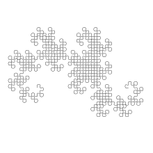
A dragon curve is any member of a family of self-similar fractal curves, which can be approximated by recursive methods such as Lindenmayer systems. The dragon curve is probably most commonly thought of as the shape that is generated from repeatedly folding a strip of paper in half, although there are other curves that are called dragon curves that are generated differently.
Heighway dragon

The Heighway dragon (also known as the Harter–Heighway dragon or the Jurassic Park dragon) was first investigated by NASA physicists John Heighway, Bruce Banks, and William Harter. It was described by Martin Gardner in his Scientific American column Mathematical Games in 1967. Many of its properties were first published by Chandler Davis and Donald Knuth. It appeared on the section title pages of the Michael Crichton novel Jurassic Park.
Construction
It can be written as a Lindenmayer system with
- angle 90°
- initial string FX
- string rewriting rules
- X ↦ X+YF+
- Y ↦ −FX−Y.
That can be described this way: starting from a base segment, replace each segment by 2 segments with a right angle and with a rotation of 45° alternatively to the right and to the left:
.svg.png)
The Heighway dragon is also the limit set of the following iterated function system in the complex plane:


with the initial set of points .

Using pairs of real numbers instead, this is the same as the two functions consisting of


This representation is more commonly used in software such as Apophysis.
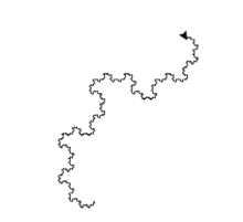
[Un]folding the dragon
Tracing an iteration of the Heighway dragon curve from one end to the other, one encounters a series of 90-degree turns, some to the right and some to the left. For the first few iterations the sequence of right (R) and left (L) turns is as follows:
- 1st iteration: R
- 2nd iteration: R R L
- 3rd iteration: R R L R R L L
- 4th iteration: R R L R R L L R R R L L R L L.
This suggests a few different patterns. First, each iteration is formed by taking the previous and adding alternating rights and lefts in between each letter. Second, it also suggests the following pattern: each iteration is formed by taking the previous iteration, adding an R at the end, and then taking the original iteration again, flipping it retrograde, swapping each letter and adding the result after the R. Due to the self-similarity exhibited by the Heighway dragon, this effectively means that each successive iteration adds a copy of the last iteration rotated counter-clockwise to the fractal.
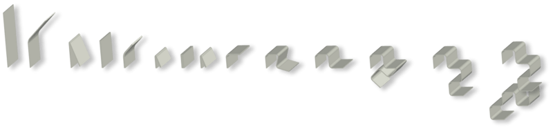
This pattern in turn suggests the following method of creating models of iterations of the Heighway dragon curve by folding a strip of paper. Take a strip of paper and fold it in half to the right. Fold it in half again to the right. If the strip was opened out now, unbending each fold to become a 90-degree turn, the turn sequence would be RRL, i.e. the second iteration of the Heighway dragon. Fold the strip in half again to the right, and the turn sequence of the unfolded strip is now RRLRRLL – the third iteration of the Heighway dragon. Continuing folding the strip in half to the right to create further iterations of the Heighway dragon (in practice, the strip becomes too thick to fold sharply after four or five iterations).
This unfolding method can be seen by calculating a number of iterations (for the animation at right, 13 iterations were used) of the curve using the "swapping" method described above, but controlling the angles for the right turns and negating prior angles.
This pattern also gives a method for determining the direction of the nth turn in the turn sequence of a Heighway dragon iteration. First, express n in the form k2m, where k is an odd number. The direction of the nth turn is determined by k mod 4, i.e. the remainder left when k is divided by 4. If k mod 4 is 1, then the nth turn is R; if k mod 4 is 3, then the nth turn is L.
For example, to determine the direction of turn 76376:
- 76376 = 9547 × 8,
- 9547 = 2386×4 + 3,
- so 9547 mod 4 = 3,
- so turn 76376 is L.
There is a simple one-line non-recursive method of implementing the above k mod 4 method of finding the turn direction in code. Treating turn n as a binary number, calculate the following boolean value:
- bool turn = (((n & −n) << 1) & n) != 0;
- "n & −n" leaves only one bit as a "1", the rightmost "1" in the binary expansion of n;
- "<< 1" shifts that bit to the left one position;
- "& n" leaves either that single bit (if k mod 4 = 3), or a zero (if k mod 4 = 1);
- so "bool turn = (((n & −n) << 1) & n) != 0" is TRUE if the nth turn is L, and is FALSE if the nth turn is R.
Gray-code method
Another way of handling this is a reduction for the above algorithm. Using Gray code, starting from zero, determine the change to the next value. If the change is a 1, then turn left, and if it is 0, then turn right. Given a binary input B, the corresponding Gray code G is given by "G = B XOR (B >> 1)". Using Gi and Gi−1, turn equals "(not Gi) AND Gi−1".
- G = B ^ (B >> 1) gets gray code from binary.
- T = (~G0) & G1: if T is equal, then to 0 turn clockwise, else turn counterclockwise.
Code
Another approach to generating this fractal can be created using a recursive function and these Turtle graphics functions drawLine(distance) and turn(angleInDegrees).
The Python code to draw an (approximate) Heighway dragon curve would look like this.
def dragon_curve(order: int, length) -> None:
    """Draw a dragon curve."""
    turn(order * 45)
    dragon_curve_recursive(order, length, 1)

def dragon_curve_recursive(order: int, length, sign) -> None:
    if order == 0:
        drawLine(length)
    else:
        rootHalf = (1 / 2) ** (1 / 2)
        dragon_curve_recursive(order - 1, length * rootHalf, 1)
        turn(sign * -90)
        dragon_curve_recursive(order - 1, length * rootHalf, -1)
Dimensions
- In spite of its strange aspect, the Heighway dragon curve has simple dimensions. Note that the dimensions 1, and 1.5 are limits and not actual values.
- Its surface is also quite simple : If the initial segment equals 1, then its surface equals . This result comes from its paving properties.
- The curve never crosses itself.
- Many self-similarities can be seen in the Heighway dragon curve. The most obvious is the repetition of the same pattern tilted by 45° and with a reduction ratio of .


- Its fractal dimension can be calculated : . That makes it a space-filling curve.
- Its boundary has an infinite length, since it increases by a similar factor every iteration.
- The fractal dimension of its boundary has been approximated numerically by Chang & Zhang .[1]).

In fact it can be found analytically:[2] This is the root of the equation


Tiling
The dragon curve can tile the plane in many ways.
 1st element with 4 curves
 2nd element with 4 curves
 3rd element with 4 curves
 The dragon curve can tile itself
 1st element with 2 curves
 2nd element with 2 curves (twindragon)
 3rd element with 2 curves
 Example of plane tiling
 Example of plane tiling
 Example of plane tiling
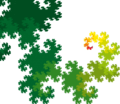 Dragon curves of increasing sizes (ratio sqrt(2)) form an infinite spiral. 4 of these spirals (with rotation 90°) tile the plane.
Twindragon
The twindragon (also known as the Davis-Knuth dragon) can be constructed by placing two Heighway dragon curves back to back. It is also the limit set of the following iterated function system:

where the initial shape is defined by the following set .

It can be also written as a Lindenmayer system – it only needs adding another section in initial string:
- angle 90°
- initial string FX+FX+
- string rewriting rules
- X ↦ X+YF
- Y ↦ FX−Y.
.jpg) Twindragon curve. |
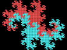 Twindragon curve constructed from two Heighway dragons. |
Terdragon

The terdragon can be written as a Lindenmayer system:
- angle 120°
- initial string F
- string rewriting rules
- F ↦ F+F−F.
It is the limit set of the following iterated function system:


.jpg)
Variants
It is possible to change the turn angle from 90° to other angles. Changing to 120° yields a structure of triangles, while 60° gives the following curve:
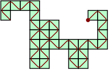
A discrete dragon curve can be converted to a dragon polyomino as shown. Like discrete dragon curves, dragon polyominoes approach the fractal dragon curve as a limit.
Occurrences of the dragon curve in solution sets
Having obtained the set of solutions to a linear differential equation, any linear combination of the solutions will, because of the superposition principle, also obey the original equation. In other words, new solutions are obtained by applying a function to the set of existing solutions. This is similar to how an iterated function system produces new points in a set, though not all IFS are linear functions. In a conceptually similar vein, a set of Littlewood polynomials can be arrived at by such iterated applications of a set of functions.
A Littlewood polynomial is a polynomial: where all .


For some we define the following functions:


Starting at z=0 we can generate all Littlewood polynomials of degree d using these functions iteratively d+1 times.[4] For instance:

It can be seen that for , the above pair of functions is equivalent to the IFS formulation of the Heighway dragon. That is, the Heighway dragon, iterated to a certain iteration, describe the set of all Littlewood polynomials up to a certain degree, evaluated at the point . Indeed, when plotting a sufficiently high number of roots of the Littlewood polynomials, structures similar to the dragon curve appear at points close to these coordinates.[4][5][6]

Notes
- Fractal dimension of the boundary of the Dragon curve
- "The Boundary of Periodic Iterated Function Systems" by Jarek Duda, The Wolfram Demonstrations Project. Recurrent construction of the boundary of dragon curve.
- Bailey, Scott; Kim, Theodore; Strichartz, Robert S. (2002), "Inside the Lévy dragon", The American Mathematical Monthly, 109 (8): 689–703, doi:10.2307/3072395, MR 1927621.
- http://golem.ph.utexas.edu/category/2009/12/this_weeks_finds_in_mathematic_46.html
- http://math.ucr.edu/home/baez/week285.html
- http://johncarlosbaez.wordpress.com/2011/12/11/the-beauty-of-roots/
Further reading
- Angel Chang; Tianrong Zhang (1999–2000). "The Fractal Geometry of the Boundary of Dragon Curves". J. Recreational Mathematics. 30 (1): 9–22.
External links
| Wikimedia Commons has media related to Dragon curve. |
- Dragon Curve—from MathWorld
- Tile made by David Chow
- Twin dragon tile with JAVA
- Eastaway, Rob. "Dragon Curves". Numberphile. Brady Haran.
- Bernard, Pierre (animation); Stewart, Alan (music). "Dragon Curve to Music". Numberphile. Brady Haran.
- Knuth on the Dragon Curve
| Characteristics |    | |
|---|---|---|
| Iterated function system | ||
| Strange attractor | ||
| L-system | ||
| Escape-time fractals | ||
| Rendering techniques | ||
| Random fractals | ||
| People | ||
| Other | ||