Convolutional neural network
In deep learning, a convolutional neural network (CNN, or ConvNet) is a class of deep neural networks, most commonly applied to analyzing visual imagery.[1] They are also known as shift invariant or space invariant artificial neural networks (SIANN), based on their shared-weights architecture and translation invariance characteristics.[2][3] They have applications in image and video recognition, recommender systems,[4] image classification, medical image analysis, natural language processing,[5] and financial time series.[6]
| Part of a series on |
| Machine learning and data mining |
|---|
 |
|
Theory |
|
Machine-learning venues |
CNNs are regularized versions of multilayer perceptrons. Multilayer perceptrons usually mean fully connected networks, that is, each neuron in one layer is connected to all neurons in the next layer. The "fully-connectedness" of these networks makes them prone to overfitting data. Typical ways of regularization include adding some form of magnitude measurement of weights to the loss function. CNNs take a different approach towards regularization: they take advantage of the hierarchical pattern in data and assemble more complex patterns using smaller and simpler patterns. Therefore, on the scale of connectedness and complexity, CNNs are on the lower extreme.
Convolutional networks were inspired by biological processes[7][8][9][10] in that the connectivity pattern between neurons resembles the organization of the animal visual cortex. Individual cortical neurons respond to stimuli only in a restricted region of the visual field known as the receptive field. The receptive fields of different neurons partially overlap such that they cover the entire visual field.
CNNs use relatively little pre-processing compared to other image classification algorithms. This means that the network learns the filters that in traditional algorithms were hand-engineered. This independence from prior knowledge and human effort in feature design is a major advantage.
Definition
The name “convolutional neural network” indicates that the network employs a mathematical operation called convolution. Convolution is a specialized kind of linear operation. Convolutional networks are simply neural networks that use convolution in place of general matrix multiplication in at least one of their layers.[11]
Architecture
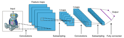
A convolutional neural network consists of an input and an output layer, as well as multiple hidden layers. The hidden layers of a CNN typically consist of a series of convolutional layers that convolve with a multiplication or other dot product. The activation function is commonly a RELU layer, and is subsequently followed by additional convolutions such as pooling layers, fully connected layers and normalization layers, referred to as hidden layers because their inputs and outputs are masked by the activation function and final convolution.
Though the layers are colloquially referred to as convolutions, this is only by convention. Mathematically, it is technically a sliding dot product or cross-correlation. This has significance for the indices in the matrix, in that it affects how weight is determined at a specific index point.
Convolutional
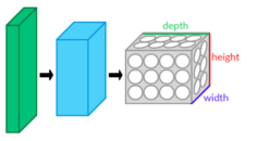
When programming a CNN, the input is a tensor with shape (number of images) x (image height) x (image width) x (image depth). Then after passing through a convolutional layer, the image becomes abstracted to a feature map, with shape (number of images) x (feature map height) x (feature map width) x (feature map channels). A convolutional layer within a neural network should have the following attributes:
- Convolutional kernels defined by a width and height (hyper-parameters).
- The number of input channels and output channels (hyper-parameter).
- The depth of the Convolution filter (the input channels) must be equal to the number channels (depth) of the input feature map.
Convolutional layers convolve the input and pass its result to the next layer. This is similar to the response of a neuron in the visual cortex to a specific stimulus.[12] Each convolutional neuron processes data only for its receptive field. Although fully connected feedforward neural networks can be used to learn features as well as classify data, it is not practical to apply this architecture to images. A very high number of neurons would be necessary, even in a shallow (opposite of deep) architecture, due to the very large input sizes associated with images, where each pixel is a relevant variable. For instance, a fully connected layer for a (small) image of size 100 x 100 has 10,000 weights for each neuron in the second layer. The convolution operation brings a solution to this problem as it reduces the number of free parameters, allowing the network to be deeper with fewer parameters.[13] For instance, regardless of image size, tiling regions of size 5 x 5, each with the same shared weights, requires only 25 learnable parameters. By using regularized weights over fewer parameters, the vanishing gradient and exploding gradient problems seen during backpropagation in traditional neural networks are avoided.[14][15]
Pooling
Convolutional networks may include local or global pooling layers to streamline the underlying computation. Pooling layers reduce the dimensions of the data by combining the outputs of neuron clusters at one layer into a single neuron in the next layer. Local pooling combines small clusters, typically 2 x 2. Global pooling acts on all the neurons of the convolutional layer.[16][17] In addition, pooling may compute a max or an average. Max pooling uses the maximum value from each of a cluster of neurons at the prior layer.[18][19] Average pooling uses the average value from each of a cluster of neurons at the prior layer.[20]
Fully connected
Fully connected layers connect every neuron in one layer to every neuron in another layer. It is in principle the same as the traditional multi-layer perceptron neural network (MLP). The flattened matrix goes through a fully connected layer to classify the images.
Receptive field
In neural networks, each neuron receives input from some number of locations in the previous layer. In a fully connected layer, each neuron receives input from every element of the previous layer. In a convolutional layer, neurons receive input from only a restricted subarea of the previous layer. Typically the subarea is of a square shape (e.g., size 5 by 5). The input area of a neuron is called its receptive field. So, in a fully connected layer, the receptive field is the entire previous layer. In a convolutional layer, the receptive area is smaller than the entire previous layer. The subarea of the original input image in the receptive field is increasingly growing as getting deeper in the network architecture. This is due to applying over and over again a convolution which takes into account the value of a specific pixel, but also some surrounding pixels.
Weights
Each neuron in a neural network computes an output value by applying a specific function to the input values coming from the receptive field in the previous layer. The function that is applied to the input values is determined by a vector of weights and a bias (typically real numbers). Learning, in a neural network, progresses by making iterative adjustments to these biases and weights.
The vector of weights and the bias are called filters and represent particular features of the input (e.g., a particular shape). A distinguishing feature of CNNs is that many neurons can share the same filter. This reduces memory footprint because a single bias and a single vector of weights are used across all receptive fields sharing that filter, as opposed to each receptive field having its own bias and vector weighting.[21]
History
CNN design follows vision processing in living organisms.
Receptive fields in the visual cortex
Work by Hubel and Wiesel in the 1950s and 1960s showed that cat and monkey visual cortexes contain neurons that individually respond to small regions of the visual field. Provided the eyes are not moving, the region of visual space within which visual stimuli affect the firing of a single neuron is known as its receptive field. Neighboring cells have similar and overlapping receptive fields. Receptive field size and location varies systematically across the cortex to form a complete map of visual space. The cortex in each hemisphere represents the contralateral visual field.
Their 1968 paper identified two basic visual cell types in the brain:[8]
- simple cells, whose output is maximized by straight edges having particular orientations within their receptive field
- complex cells, which have larger receptive fields, whose output is insensitive to the exact position of the edges in the field.
Hubel and Wiesel also proposed a cascading model of these two types of cells for use in pattern recognition tasks.[22][23]
Neocognitron, origin of the CNN architecture
The "neocognitron"[7] was introduced by Kunihiko Fukushima in 1980.[9][19][24] It was inspired by the above-mentioned work of Hubel and Wiesel. The neocognitron introduced the two basic types of layers in CNNs: convolutional layers, and downsampling layers. A convolutional layer contains units whose receptive fields cover a patch of the previous layer. The weight vector (the set of adaptive parameters) of such a unit is often called a filter. Units can share filters. Downsampling layers contain units whose receptive fields cover patches of previous convolutional layers. Such a unit typically computes the average of the activations of the units in its patch. This downsampling helps to correctly classify objects in visual scenes even when the objects are shifted.
In a variant of the neocognitron called the cresceptron, instead of using Fukushima's spatial averaging, J. Weng et al. introduced a method called max-pooling where a downsampling unit computes the maximum of the activations of the units in its patch.[25] Max-pooling is often used in modern CNNs.[26]
Several supervised and unsupervised learning algorithms have been proposed over the decades to train the weights of a neocognitron.[7] Today, however, the CNN architecture is usually trained through backpropagation.
The neocognitron is the first CNN which requires units located at multiple network positions to have shared weights. Neocognitrons were adapted in 1988 to analyze time-varying signals.[27]
Time delay neural networks
The time delay neural network (TDNN) was introduced in 1987 by Alex Waibel et al. and was the first convolutional network, as it achieved shift invariance.[28] It did so by utilizing weight sharing in combination with Backpropagation training.[29] Thus, while also using a pyramidal structure as in the neocognitron, it performed a global optimization of the weights instead of a local one.[28]
TDNNs are convolutional networks that share weights along the temporal dimension.[30] They allow speech signals to be processed time-invariantly. In 1990 Hampshire and Waibel introduced a variant which performs a two dimensional convolution.[31] Since these TDNNs operated on spectrograms, the resulting phoneme recognition system was invariant to both shifts in time and in frequency. This inspired translation invariance in image processing with CNNs.[29] The tiling of neuron outputs can cover timed stages.[32]
TDNNs now achieve the best performance in far distance speech recognition.[33]
Max pooling
In 1990 Yamaguchi et al. introduced the concept of max pooling. They did so by combining TDNNs with max pooling in order to realize a speaker independent isolated word recognition system.[18] In their system they used several TDNNs per word, one for each syllable. The results of each TDNN over the input signal were combined using max pooling and the outputs of the pooling layers were then passed on to networks performing the actual word classification.
Image recognition with CNNs trained by gradient descent
A system to recognize hand-written ZIP Code numbers[34] involved convolutions in which the kernel coefficients had been laboriously hand designed.[35]
Yann LeCun et al. (1989)[35] used back-propagation to learn the convolution kernel coefficients directly from images of hand-written numbers. Learning was thus fully automatic, performed better than manual coefficient design, and was suited to a broader range of image recognition problems and image types.
This approach became a foundation of modern computer vision.
LeNet-5
LeNet-5, a pioneering 7-level convolutional network by LeCun et al. in 1998,[36] that classifies digits, was applied by several banks to recognize hand-written numbers on checks (British English: cheques) digitized in 32x32 pixel images. The ability to process higher resolution images requires larger and more layers of convolutional neural networks, so this technique is constrained by the availability of computing resources.
Shift-invariant neural network
Similarly, a shift invariant neural network was proposed by W. Zhang et al. for image character recognition in 1988.[2][3] The architecture and training algorithm were modified in 1991[37] and applied for medical image processing[38] and automatic detection of breast cancer in mammograms.[39]
A different convolution-based design was proposed in 1988[40] for application to decomposition of one-dimensional electromyography convolved signals via de-convolution. This design was modified in 1989 to other de-convolution-based designs.[41][42]
Neural abstraction pyramid

The feed-forward architecture of convolutional neural networks was extended in the neural abstraction pyramid[43] by lateral and feedback connections. The resulting recurrent convolutional network allows for the flexible incorporation of contextual information to iteratively resolve local ambiguities. In contrast to previous models, image-like outputs at the highest resolution were generated, e.g., for semantic segmentation, image reconstruction, and object localization tasks.
GPU implementations
Although CNNs were invented in the 1980s, their breakthrough in the 2000s required fast implementations on graphics processing units (GPUs).
In 2004, it was shown by K. S. Oh and K. Jung that standard neural networks can be greatly accelerated on GPUs. Their implementation was 20 times faster than an equivalent implementation on CPU.[44][26] In 2005, another paper also emphasised the value of GPGPU for machine learning.[45]
The first GPU-implementation of a CNN was described in 2006 by K. Chellapilla et al. Their implementation was 4 times faster than an equivalent implementation on CPU.[46] Subsequent work also used GPUs, initially for other types of neural networks (different from CNNs), especially unsupervised neural networks.[47][48][49][50]
In 2010, Dan Ciresan et al. at IDSIA showed that even deep standard neural networks with many layers can be quickly trained on GPU by supervised learning through the old method known as backpropagation. Their network outperformed previous machine learning methods on the MNIST handwritten digits benchmark.[51] In 2011, they extended this GPU approach to CNNs, achieving an acceleration factor of 60, with impressive results.[16] In 2011, they used such CNNs on GPU to win an image recognition contest where they achieved superhuman performance for the first time.[52] Between May 15, 2011 and September 30, 2012, their CNNs won no less than four image competitions.[53][26] In 2012, they also significantly improved on the best performance in the literature for multiple image databases, including the MNIST database, the NORB database, the HWDB1.0 dataset (Chinese characters) and the CIFAR10 dataset (dataset of 60000 32x32 labeled RGB images).[19]
Subsequently, a similar GPU-based CNN by Alex Krizhevsky et al. won the ImageNet Large Scale Visual Recognition Challenge 2012.[54] A very deep CNN with over 100 layers by Microsoft won the ImageNet 2015 contest.[55]
Intel Xeon Phi implementations
Compared to the training of CNNs using GPUs, not much attention was given to the Intel Xeon Phi coprocessor.[56] A notable development is a parallelization method for training convolutional neural networks on the Intel Xeon Phi, named Controlled Hogwild with Arbitrary Order of Synchronization (CHAOS).[57] CHAOS exploits both the thread- and SIMD-level parallelism that is available on the Intel Xeon Phi.
Distinguishing features
In the past, traditional multilayer perceptron (MLP) models have been used for image recognition. However, due to the full connectivity between nodes, they suffered from the curse of dimensionality, and did not scale well with higher resolution images. A 1000×1000-pixel image with RGB color channels has 3 million weights, which is too high to feasibly process efficiently at scale with full connectivity.
For example, in CIFAR-10, images are only of size 32×32×3 (32 wide, 32 high, 3 color channels), so a single fully connected neuron in a first hidden layer of a regular neural network would have 32*32*3 = 3,072 weights. A 200×200 image, however, would lead to neurons that have 200*200*3 = 120,000 weights.
Also, such network architecture does not take into account the spatial structure of data, treating input pixels which are far apart in the same way as pixels that are close together. This ignores locality of reference in image data, both computationally and semantically. Thus, full connectivity of neurons is wasteful for purposes such as image recognition that are dominated by spatially local input patterns.
Convolutional neural networks are biologically inspired variants of multilayer perceptrons that are designed to emulate the behavior of a visual cortex. These models mitigate the challenges posed by the MLP architecture by exploiting the strong spatially local correlation present in natural images. As opposed to MLPs, CNNs have the following distinguishing features:
- 3D volumes of neurons. The layers of a CNN have neurons arranged in 3 dimensions: width, height and depth. where each neuron inside a convolutional layer is connected to only a small region of the layer before it, called a receptive field. Distinct types of layers, both locally and completely connected, are stacked to form a CNN architecture.
- Local connectivity: following the concept of receptive fields, CNNs exploit spatial locality by enforcing a local connectivity pattern between neurons of adjacent layers. The architecture thus ensures that the learned "filters" produce the strongest response to a spatially local input pattern. Stacking many such layers leads to non-linear filters that become increasingly global (i.e. responsive to a larger region of pixel space) so that the network first creates representations of small parts of the input, then from them assembles representations of larger areas.
- Shared weights: In CNNs, each filter is replicated across the entire visual field. These replicated units share the same parameterization (weight vector and bias) and form a feature map. This means that all the neurons in a given convolutional layer respond to the same feature within their specific response field. Replicating units in this way allows for the resulting feature map to be equivariant under changes in the locations of input features in the visual field, i.e. they grant translational equivariance.
- Pooling: In a CNN's pooling layers, feature maps are divided into rectangular sub-regions, and the features in each rectangle are independently down-sampled to a single value, commonly by taking their average or maximum value. In addition to reducing the sizes of feature maps, the pooling operation grants a degree of translational invariance to the features contained therein, allowing the CNN to be more robust to variations in their positions.
Together, these properties allow CNNs to achieve better generalization on vision problems. Weight sharing dramatically reduces the number of free parameters learned, thus lowering the memory requirements for running the network and allowing the training of larger, more powerful networks.
Building blocks
A CNN architecture is formed by a stack of distinct layers that transform the input volume into an output volume (e.g. holding the class scores) through a differentiable function. A few distinct types of layers are commonly used. These are further discussed below.

Convolutional layer
The convolutional layer is the core building block of a CNN. The layer's parameters consist of a set of learnable filters (or kernels), which have a small receptive field, but extend through the full depth of the input volume. During the forward pass, each filter is convolved across the width and height of the input volume, computing the dot product between the entries of the filter and the input and producing a 2-dimensional activation map of that filter. As a result, the network learns filters that activate when it detects some specific type of feature at some spatial position in the input.[nb 1]
Stacking the activation maps for all filters along the depth dimension forms the full output volume of the convolution layer. Every entry in the output volume can thus also be interpreted as an output of a neuron that looks at a small region in the input and shares parameters with neurons in the same activation map.
Local connectivity
When dealing with high-dimensional inputs such as images, it is impractical to connect neurons to all neurons in the previous volume because such a network architecture does not take the spatial structure of the data into account. Convolutional networks exploit spatially local correlation by enforcing a sparse local connectivity pattern between neurons of adjacent layers: each neuron is connected to only a small region of the input volume.
The extent of this connectivity is a hyperparameter called the receptive field of the neuron. The connections are local in space (along width and height), but always extend along the entire depth of the input volume. Such an architecture ensures that the learnt filters produce the strongest response to a spatially local input pattern.
Spatial arrangement
Three hyperparameters control the size of the output volume of the convolutional layer: the depth, stride and zero-padding.
- The depth of the output volume controls the number of neurons in a layer that connect to the same region of the input volume. These neurons learn to activate for different features in the input. For example, if the first convolutional layer takes the raw image as input, then different neurons along the depth dimension may activate in the presence of various oriented edges, or blobs of color.
- Stride controls how depth columns around the spatial dimensions (width and height) are allocated. When the stride is 1 then we move the filters one pixel at a time. This leads to heavily overlapping receptive fields between the columns, and also to large output volumes. When the stride is 2 then the filters jump 2 pixels at a time as they slide around. Similarly, for any integer a stride of S causes the filter to be translated by S units at a time per output. In practice, stride lengths of are rare. The receptive fields overlap less and the resulting output volume has smaller spatial dimensions when stride length is increased.[58]
- Sometimes it is convenient to pad the input with zeros on the border of the input volume. The size of this padding is a third hyperparameter. Padding provides control of the output volume spatial size. In particular, sometimes it is desirable to exactly preserve the spatial size of the input volume.


The spatial size of the output volume can be computed as a function of the input volume size , the kernel field size of the convolutional layer neurons , the stride with which they are applied , and the amount of zero padding used on the border. The formula for calculating how many neurons "fit" in a given volume is given by


If this number is not an integer, then the strides are incorrect and the neurons cannot be tiled to fit across the input volume in a symmetric way. In general, setting zero padding to be when the stride is ensures that the input volume and output volume will have the same size spatially. However, it's not always completely necessary to use all of the neurons of the previous layer. For example, a neural network designer may decide to use just a portion of padding.


Parameter sharing
A parameter sharing scheme is used in convolutional layers to control the number of free parameters. It relies on the assumption that if a patch feature is useful to compute at some spatial position, then it should also be useful to compute at other positions. Denoting a single 2-dimensional slice of depth as a depth slice, the neurons in each depth slice are constrained to use the same weights and bias.
Since all neurons in a single depth slice share the same parameters, the forward pass in each depth slice of the convolutional layer can be computed as a convolution of the neuron's weights with the input volume.[nb 2] Therefore, it is common to refer to the sets of weights as a filter (or a kernel), which is convolved with the input. The result of this convolution is an activation map, and the set of activation maps for each different filter are stacked together along the depth dimension to produce the output volume. Parameter sharing contributes to the translation invariance of the CNN architecture.
Sometimes, the parameter sharing assumption may not make sense. This is especially the case when the input images to a CNN have some specific centered structure; for which we expect completely different features to be learned on different spatial locations. One practical example is when the inputs are faces that have been centered in the image: we might expect different eye-specific or hair-specific features to be learned in different parts of the image. In that case it is common to relax the parameter sharing scheme, and instead simply call the layer a "locally connected layer".
Pooling layer
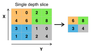
Another important concept of CNNs is pooling, which is a form of non-linear down-sampling. There are several non-linear functions to implement pooling among which max pooling is the most common. It partitions the input image into a set of non-overlapping rectangles and, for each such sub-region, outputs the maximum.
Intuitively, the exact location of a feature is less important than its rough location relative to other features. This is the idea behind the use of pooling in convolutional neural networks. The pooling layer serves to progressively reduce the spatial size of the representation, to reduce the number of parameters, memory footprint and amount of computation in the network, and hence to also control overfitting. It is common to periodically insert a pooling layer between successive convolutional layers in a CNN architecture. The pooling operation provides another form of translation invariance.
The pooling layer operates independently on every depth slice of the input and resizes it spatially. The most common form is a pooling layer with filters of size 2×2 applied with a stride of 2 downsamples at every depth slice in the input by 2 along both width and height, discarding 75% of the activations:

In this case, every max operation is over 4 numbers. The depth dimension remains unchanged.
In addition to max pooling, pooling units can use other functions, such as average pooling or ℓ2-norm pooling. Average pooling was often used historically but has recently fallen out of favor compared to max pooling, which performs better in practice.[59]
Due to the aggressive reduction in the size of the representation, there is a recent trend towards using smaller filters[60] or discarding pooling layers altogether.[61]
"Region of Interest" pooling (also known as RoI pooling) is a variant of max pooling, in which output size is fixed and input rectangle is a parameter.[62]
Pooling is an important component of convolutional neural networks for object detection based on Fast R-CNN[63] architecture.
ReLU layer
ReLU is the abbreviation of rectified linear unit, which applies the non-saturating activation function .[54] It effectively removes negative values from an activation map by setting them to zero.[64] It increases the nonlinear properties of the decision function and of the overall network without affecting the receptive fields of the convolution layer.

Other functions are also used to increase nonlinearity, for example the saturating hyperbolic tangent , , and the sigmoid function . ReLU is often preferred to other functions because it trains the neural network several times faster without a significant penalty to generalization accuracy.[65]


Fully connected layer
Finally, after several convolutional and max pooling layers, the high-level reasoning in the neural network is done via fully connected layers. Neurons in a fully connected layer have connections to all activations in the previous layer, as seen in regular (non-convolutional) artificial neural networks. Their activations can thus be computed as an affine transformation, with matrix multiplication followed by a bias offset (vector addition of a learned or fixed bias term).
Loss layer
The "loss layer" specifies how training penalizes the deviation between the predicted (output) and true labels and is normally the final layer of a neural network. Various loss functions appropriate for different tasks may be used.
Softmax loss is used for predicting a single class of K mutually exclusive classes.[nb 3] Sigmoid cross-entropy loss is used for predicting K independent probability values in . Euclidean loss is used for regressing to real-valued labels .


Choosing hyperparameters
CNNs use more hyperparameters than a standard multilayer perceptron (MLP). While the usual rules for learning rates and regularization constants still apply, the following should be kept in mind when optimizing.
Number of filters
Since feature map size decreases with depth, layers near the input layer will tend to have fewer filters while higher layers can have more. To equalize computation at each layer, the product of feature values va with pixel position is kept roughly constant across layers. Preserving more information about the input would require keeping the total number of activations (number of feature maps times number of pixel positions) non-decreasing from one layer to the next.
The number of feature maps directly controls the capacity and depends on the number of available examples and task complexity.
Filter shape
Common filter shapes found in the literature vary greatly, and are usually chosen based on the dataset.
The challenge is, thus, to find the right level of granularity so as to create abstractions at the proper scale, given a particular dataset, and without overfitting.
Max pooling shape
Typical values are 2×2. Very large input volumes may warrant 4×4 pooling in the lower layers.[66] However, choosing larger shapes will dramatically reduce the dimension of the signal, and may result in excess information loss. Often, non-overlapping pooling windows perform best.[59]
Regularization methods
Regularization is a process of introducing additional information to solve an ill-posed problem or to prevent overfitting. CNNs use various types of regularization.
Empirical
Dropout
Because a fully connected layer occupies most of the parameters, it is prone to overfitting. One method to reduce overfitting is dropout.[67][68] At each training stage, individual nodes are either "dropped out" of the net with probability or kept with probability , so that a reduced network is left; incoming and outgoing edges to a dropped-out node are also removed. Only the reduced network is trained on the data in that stage. The removed nodes are then reinserted into the network with their original weights.


In the training stages, the probability that a hidden node will be dropped is usually 0.5; for input nodes, however, this probability is typically much lower, since information is directly lost when input nodes are ignored or dropped.
At testing time after training has finished, we would ideally like to find a sample average of all possible dropped-out networks; unfortunately this is unfeasible for large values of . However, we can find an approximation by using the full network with each node's output weighted by a factor of , so the expected value of the output of any node is the same as in the training stages. This is the biggest contribution of the dropout method: although it effectively generates neural nets, and as such allows for model combination, at test time only a single network needs to be tested.


By avoiding training all nodes on all training data, dropout decreases overfitting. The method also significantly improves training speed. This makes the model combination practical, even for deep neural networks. The technique seems to reduce node interactions, leading them to learn more robust features that better generalize to new data.
DropConnect
DropConnect is the generalization of dropout in which each connection, rather than each output unit, can be dropped with probability . Each unit thus receives input from a random subset of units in the previous layer.[69]
DropConnect is similar to dropout as it introduces dynamic sparsity within the model, but differs in that the sparsity is on the weights, rather than the output vectors of a layer. In other words, the fully connected layer with DropConnect becomes a sparsely connected layer in which the connections are chosen at random during the training stage.
Stochastic pooling
A major drawback to Dropout is that it does not have the same benefits for convolutional layers, where the neurons are not fully connected.
In stochastic pooling,[70] the conventional deterministic pooling operations are replaced with a stochastic procedure, where the activation within each pooling region is picked randomly according to a multinomial distribution, given by the activities within the pooling region. This approach is free of hyperparameters and can be combined with other regularization approaches, such as dropout and data augmentation.
An alternate view of stochastic pooling is that it is equivalent to standard max pooling but with many copies of an input image, each having small local deformations. This is similar to explicit elastic deformations of the input images,[71] which delivers excellent performance on the MNIST data set.[71] Using stochastic pooling in a multilayer model gives an exponential number of deformations since the selections in higher layers are independent of those below.
Artificial data
Since the degree of model overfitting is determined by both its power and the amount of training it receives, providing a convolutional network with more training examples can reduce overfitting. Since these networks are usually trained with all available data, one approach is to either generate new data from scratch (if possible) or perturb existing data to create new ones. For example, input images could be asymmetrically cropped by a few percent to create new examples with the same label as the original.[72]
Explicit
Early stopping
One of the simplest methods to prevent overfitting of a network is to simply stop the training before overfitting has had a chance to occur. It comes with the disadvantage that the learning process is halted.
Number of parameters
Another simple way to prevent overfitting is to limit the number of parameters, typically by limiting the number of hidden units in each layer or limiting network depth. For convolutional networks, the filter size also affects the number of parameters. Limiting the number of parameters restricts the predictive power of the network directly, reducing the complexity of the function that it can perform on the data, and thus limits the amount of overfitting. This is equivalent to a "zero norm".
Weight decay
A simple form of added regularizer is weight decay, which simply adds an additional error, proportional to the sum of weights (L1 norm) or squared magnitude (L2 norm) of the weight vector, to the error at each node. The level of acceptable model complexity can be reduced by increasing the proportionality constant, thus increasing the penalty for large weight vectors.
L2 regularization is the most common form of regularization. It can be implemented by penalizing the squared magnitude of all parameters directly in the objective. The L2 regularization has the intuitive interpretation of heavily penalizing peaky weight vectors and preferring diffuse weight vectors. Due to multiplicative interactions between weights and inputs this has the useful property of encouraging the network to use all of its inputs a little rather than some of its inputs a lot.
L1 regularization is another common form. It is possible to combine L1 with L2 regularization (this is called Elastic net regularization). The L1 regularization leads the weight vectors to become sparse during optimization. In other words, neurons with L1 regularization end up using only a sparse subset of their most important inputs and become nearly invariant to the noisy inputs.
Max norm constraints
Another form of regularization is to enforce an absolute upper bound on the magnitude of the weight vector for every neuron and use projected gradient descent to enforce the constraint. In practice, this corresponds to performing the parameter update as normal, and then enforcing the constraint by clamping the weight vector of every neuron to satisfy . Typical values of are order of 3–4. Some papers report improvements[73] when using this form of regularization.


Hierarchical coordinate frames
Pooling loses the precise spatial relationships between high-level parts (such as nose and mouth in a face image). These relationships are needed for identity recognition. Overlapping the pools so that each feature occurs in multiple pools, helps retain the information. Translation alone cannot extrapolate the understanding of geometric relationships to a radically new viewpoint, such as a different orientation or scale. On the other hand, people are very good at extrapolating; after seeing a new shape once they can recognize it from a different viewpoint.[74]
Currently, the common way to deal with this problem is to train the network on transformed data in different orientations, scales, lighting, etc. so that the network can cope with these variations. This is computationally intensive for large data-sets. The alternative is to use a hierarchy of coordinate frames and to use a group of neurons to represent a conjunction of the shape of the feature and its pose relative to the retina. The pose relative to retina is the relationship between the coordinate frame of the retina and the intrinsic features' coordinate frame.[75]
Thus, one way of representing something is to embed the coordinate frame within it. Once this is done, large features can be recognized by using the consistency of the poses of their parts (e.g. nose and mouth poses make a consistent prediction of the pose of the whole face). Using this approach ensures that the higher level entity (e.g. face) is present when the lower level (e.g. nose and mouth) agree on its prediction of the pose. The vectors of neuronal activity that represent pose ("pose vectors") allow spatial transformations modeled as linear operations that make it easier for the network to learn the hierarchy of visual entities and generalize across viewpoints. This is similar to the way the human visual system imposes coordinate frames in order to represent shapes.[76]
Applications
Image recognition
CNNs are often used in image recognition systems. In 2012 an error rate of 0.23 percent on the MNIST database was reported.[19] Another paper on using CNN for image classification reported that the learning process was "surprisingly fast"; in the same paper, the best published results as of 2011 were achieved in the MNIST database and the NORB database.[16] Subsequently, a similar CNN called AlexNet[77] won the ImageNet Large Scale Visual Recognition Challenge 2012.
When applied to facial recognition, CNNs achieved a large decrease in error rate.[78] Another paper reported a 97.6 percent recognition rate on "5,600 still images of more than 10 subjects".[10] CNNs were used to assess video quality in an objective way after manual training; the resulting system had a very low root mean square error.[32]
The ImageNet Large Scale Visual Recognition Challenge is a benchmark in object classification and detection, with millions of images and hundreds of object classes. In the ILSVRC 2014,[79] a large-scale visual recognition challenge, almost every highly ranked team used CNN as their basic framework. The winner GoogLeNet[80] (the foundation of DeepDream) increased the mean average precision of object detection to 0.439329, and reduced classification error to 0.06656, the best result to date. Its network applied more than 30 layers. That performance of convolutional neural networks on the ImageNet tests was close to that of humans.[81] The best algorithms still struggle with objects that are small or thin, such as a small ant on a stem of a flower or a person holding a quill in their hand. They also have trouble with images that have been distorted with filters, an increasingly common phenomenon with modern digital cameras. By contrast, those kinds of images rarely trouble humans. Humans, however, tend to have trouble with other issues. For example, they are not good at classifying objects into fine-grained categories such as the particular breed of dog or species of bird, whereas convolutional neural networks handle this.
In 2015 a many-layered CNN demonstrated the ability to spot faces from a wide range of angles, including upside down, even when partially occluded, with competitive performance. The network was trained on a database of 200,000 images that included faces at various angles and orientations and a further 20 million images without faces. They used batches of 128 images over 50,000 iterations.[82]
Video analysis
Compared to image data domains, there is relatively little work on applying CNNs to video classification. Video is more complex than images since it has another (temporal) dimension. However, some extensions of CNNs into the video domain have been explored. One approach is to treat space and time as equivalent dimensions of the input and perform convolutions in both time and space.[83][84] Another way is to fuse the features of two convolutional neural networks, one for the spatial and one for the temporal stream.[85][86][87] Long short-term memory (LSTM) recurrent units are typically incorporated after the CNN to account for inter-frame or inter-clip dependencies.[88][89] Unsupervised learning schemes for training spatio-temporal features have been introduced, based on Convolutional Gated Restricted Boltzmann Machines[90] and Independent Subspace Analysis.[91]
Natural language processing
CNNs have also been explored for natural language processing. CNN models are effective for various NLP problems and achieved excellent results in semantic parsing,[92] search query retrieval,[93] sentence modeling,[94] classification,[95] prediction[96] and other traditional NLP tasks.[97]
Anomaly Detection
A CNN with 1-D convolutions was used on time series in the frequency domain (spectral residual) by an unsupervised model to detect anomalies in the time domain.[98]
Drug discovery
CNNs have been used in drug discovery. Predicting the interaction between molecules and biological proteins can identify potential treatments. In 2015, Atomwise introduced AtomNet, the first deep learning neural network for structure-based rational drug design.[99] The system trains directly on 3-dimensional representations of chemical interactions. Similar to how image recognition networks learn to compose smaller, spatially proximate features into larger, complex structures,[100] AtomNet discovers chemical features, such as aromaticity, sp3 carbons and hydrogen bonding. Subsequently, AtomNet was used to predict novel candidate biomolecules for multiple disease targets, most notably treatments for the Ebola virus[101] and multiple sclerosis.[102]
Health risk assessment and biomarkers of aging discovery
CNNs can be naturally tailored to analyze a sufficiently large collection of time series data representing one-week-long human physical activity streams augmented by the rich clinical data (including the death register, as provided by, e.g., the NHANES study). A simple CNN was combined with Cox-Gompertz proportional hazards model and used to produce a proof-of-concept example of digital biomarkers of aging in the form of all-causes-mortality predictor.[103]
Checkers game
CNNs have been used in the game of checkers. From 1999 to 2001, Fogel and Chellapilla published papers showing how a convolutional neural network could learn to play checker using co-evolution. The learning process did not use prior human professional games, but rather focused on a minimal set of information contained in the checkerboard: the location and type of pieces, and the difference in number of pieces between the two sides. Ultimately, the program (Blondie24) was tested on 165 games against players and ranked in the highest 0.4%.[104][105] It also earned a win against the program Chinook at its "expert" level of play.[106]
Go
CNNs have been used in computer Go. In December 2014, Clark and Storkey published a paper showing that a CNN trained by supervised learning from a database of human professional games could outperform GNU Go and win some games against Monte Carlo tree search Fuego 1.1 in a fraction of the time it took Fuego to play.[107] Later it was announced that a large 12-layer convolutional neural network had correctly predicted the professional move in 55% of positions, equalling the accuracy of a 6 dan human player. When the trained convolutional network was used directly to play games of Go, without any search, it beat the traditional search program GNU Go in 97% of games, and matched the performance of the Monte Carlo tree search program Fuego simulating ten thousand playouts (about a million positions) per move.[108]
A couple of CNNs for choosing moves to try ("policy network") and evaluating positions ("value network") driving MCTS were used by AlphaGo, the first to beat the best human player at the time.[109]
Time series forecasting
Recurrent neural networks are generally considered the best neural network architectures for time series forecasting (and sequence modeling in general), but recent studies show that convolutional networks can perform comparably or even better.[110][6] Dilated convolutions[111] might enable one-dimensional convolutional neural networks to effectively learn time series dependences.[112] Convolutions can be implemented more efficiently than RNN-based solutions, and they do not suffer from vanishing (or exploding) gradients.[113] Convolutional networks can provide an improved forecasting performance when there are multiple similar time series to learn from.[114] CNNs can also be applied to further tasks in time series analysis (e.g., time series classification[115] or quantile forecasting[116]).
Fine-tuning
For many applications, the training data is less available. Convolutional neural networks usually require a large amount of training data in order to avoid overfitting. A common technique is to train the network on a larger data set from a related domain. Once the network parameters have converged an additional training step is performed using the in-domain data to fine-tune the network weights. This allows convolutional networks to be successfully applied to problems with small training sets.[117]
Human interpretable explanations
End-to-end training and prediction are common practice in computer vision. However, human interpretable explanations are required for critical systems such as a self-driving cars.[118] With recent advances in visual salience, spatial and temporal attention, the most critical spatial regions/temporal instants could be visualized to justify the CNN predictions.[119][120]
Related architectures
Deep Q-networks
A deep Q-network (DQN) is a type of deep learning model that combines a deep neural network with Q-learning, a form of reinforcement learning. Unlike earlier reinforcement learning agents, DQNs that utilize CNNs can learn directly from high-dimensional sensory inputs.
Preliminary results were presented in 2014, with an accompanying paper in February 2015.[121] The research described an application to Atari 2600 gaming. Other deep reinforcement learning models preceded it.[122]
Deep belief networks
Convolutional deep belief networks (CDBN) have structure very similar to convolutional neural networks and are trained similarly to deep belief networks. Therefore, they exploit the 2D structure of images, like CNNs do, and make use of pre-training like deep belief networks. They provide a generic structure that can be used in many image and signal processing tasks. Benchmark results on standard image datasets like CIFAR[123] have been obtained using CDBNs.[124]
Notable libraries
- Caffe: A library for convolutional neural networks. Created by the Berkeley Vision and Learning Center (BVLC). It supports both CPU and GPU. Developed in C++, and has Python and MATLAB wrappers.
- Deeplearning4j: Deep learning in Java and Scala on multi-GPU-enabled Spark. A general-purpose deep learning library for the JVM production stack running on a C++ scientific computing engine. Allows the creation of custom layers. Integrates with Hadoop and Kafka.
- Dlib: A toolkit for making real world machine learning and data analysis applications in C++.
- Microsoft Cognitive Toolkit: A deep learning toolkit written by Microsoft with several unique features enhancing scalability over multiple nodes. It supports full-fledged interfaces for training in C++ and Python and with additional support for model inference in C# and Java.
- TensorFlow: Apache 2.0-licensed Theano-like library with support for CPU, GPU, Google's proprietary tensor processing unit (TPU),[125] and mobile devices.
- Theano: The reference deep-learning library for Python with an API largely compatible with the popular NumPy library. Allows user to write symbolic mathematical expressions, then automatically generates their derivatives, saving the user from having to code gradients or backpropagation. These symbolic expressions are automatically compiled to CUDA code for a fast, on-the-GPU implementation.
- Torch: A scientific computing framework with wide support for machine learning algorithms, written in C and Lua. The main author is Ronan Collobert, and it is now used at Facebook AI Research and Twitter.
Notable APIs
- Keras: A high level API written in Python for TensorFlow and Theano convolutional neural networks.[126]
See also
- Convolution
- Deep learning
- Natural-language processing
- Neocognitron
- Scale-invariant feature transform
- Time delay neural network
- Vision processing unit
Notes
- When applied to other types of data than image data, such as sound data, "spatial position" may variously correspond to different points in the time domain, frequency domain or other mathematical spaces.
- hence the name "convolutional layer"
- So-called categorical data.
References
- Valueva, M.V.; Nagornov, N.N.; Lyakhov, P.A.; Valuev, G.V.; Chervyakov, N.I. (2020). "Application of the residue number system to reduce hardware costs of the convolutional neural network implementation". Mathematics and Computers in Simulation. Elsevier BV. 177: 232–243. doi:10.1016/j.matcom.2020.04.031. ISSN 0378-4754.
Convolutional neural networks are a promising tool for solving the problem of pattern recognition.
- Zhang, Wei (1988). "Shift-invariant pattern recognition neural network and its optical architecture". Proceedings of Annual Conference of the Japan Society of Applied Physics.
- Zhang, Wei (1990). "Parallel distributed processing model with local space-invariant interconnections and its optical architecture". Applied Optics. 29 (32): 4790–7. Bibcode:1990ApOpt..29.4790Z. doi:10.1364/AO.29.004790. PMID 20577468.
- van den Oord, Aaron; Dieleman, Sander; Schrauwen, Benjamin (2013-01-01). Burges, C. J. C.; Bottou, L.; Welling, M.; Ghahramani, Z.; Weinberger, K. Q. (eds.). Deep content-based music recommendation (PDF). Curran Associates, Inc. pp. 2643–2651.
- Collobert, Ronan; Weston, Jason (2008-01-01). A Unified Architecture for Natural Language Processing: Deep Neural Networks with Multitask Learning. Proceedings of the 25th International Conference on Machine Learning. ICML '08. New York, NY, USA: ACM. pp. 160–167. doi:10.1145/1390156.1390177. ISBN 978-1-60558-205-4.
- Tsantekidis, Avraam; Passalis, Nikolaos; Tefas, Anastasios; Kanniainen, Juho; Gabbouj, Moncef; Iosifidis, Alexandros (July 2017). "Forecasting Stock Prices from the Limit Order Book Using Convolutional Neural Networks". 2017 IEEE 19th Conference on Business Informatics (CBI). Thessaloniki, Greece: IEEE: 7–12. doi:10.1109/CBI.2017.23. ISBN 978-1-5386-3035-8.
- Fukushima, K. (2007). "Neocognitron". Scholarpedia. 2 (1): 1717. Bibcode:2007SchpJ...2.1717F. doi:10.4249/scholarpedia.1717.
- Hubel, D. H.; Wiesel, T. N. (1968-03-01). "Receptive fields and functional architecture of monkey striate cortex". The Journal of Physiology. 195 (1): 215–243. doi:10.1113/jphysiol.1968.sp008455. ISSN 0022-3751. PMC 1557912. PMID 4966457.
- Fukushima, Kunihiko (1980). "Neocognitron: A Self-organizing Neural Network Model for a Mechanism of Pattern Recognition Unaffected by Shift in Position" (PDF). Biological Cybernetics. 36 (4): 193–202. doi:10.1007/BF00344251. PMID 7370364. Retrieved 16 November 2013.
- Matusugu, Masakazu; Katsuhiko Mori; Yusuke Mitari; Yuji Kaneda (2003). "Subject independent facial expression recognition with robust face detection using a convolutional neural network" (PDF). Neural Networks. 16 (5): 555–559. doi:10.1016/S0893-6080(03)00115-1. PMID 12850007. Retrieved 17 November 2013.
- Ian Goodfellow and Yoshua Bengio and Aaron Courville (2016). Deep Learning. MIT Press. p. 326.
- "Convolutional Neural Networks (LeNet) – DeepLearning 0.1 documentation". DeepLearning 0.1. LISA Lab. Retrieved 31 August 2013.
- Habibi, Aghdam, Hamed (2017-05-30). Guide to convolutional neural networks : a practical application to traffic-sign detection and classification. Heravi, Elnaz Jahani. Cham, Switzerland. ISBN 9783319575490. OCLC 987790957.
- Venkatesan, Ragav; Li, Baoxin (2017-10-23). Convolutional Neural Networks in Visual Computing: A Concise Guide. CRC Press. ISBN 978-1-351-65032-8.
- Balas, Valentina E.; Kumar, Raghvendra; Srivastava, Rajshree (2019-11-19). Recent Trends and Advances in Artificial Intelligence and Internet of Things. Springer Nature. ISBN 978-3-030-32644-9.
- Ciresan, Dan; Ueli Meier; Jonathan Masci; Luca M. Gambardella; Jurgen Schmidhuber (2011). "Flexible, High Performance Convolutional Neural Networks for Image Classification" (PDF). Proceedings of the Twenty-Second International Joint Conference on Artificial Intelligence-Volume Volume Two. 2: 1237–1242. Retrieved 17 November 2013.
- Krizhevsky, Alex. "ImageNet Classification with Deep Convolutional Neural Networks" (PDF). Retrieved 17 November 2013.
- Yamaguchi, Kouichi; Sakamoto, Kenji; Akabane, Toshio; Fujimoto, Yoshiji (November 1990). A Neural Network for Speaker-Independent Isolated Word Recognition. First International Conference on Spoken Language Processing (ICSLP 90). Kobe, Japan.
- Ciresan, Dan; Meier, Ueli; Schmidhuber, Jürgen (June 2012). Multi-column deep neural networks for image classification. 2012 IEEE Conference on Computer Vision and Pattern Recognition. New York, NY: Institute of Electrical and Electronics Engineers (IEEE). pp. 3642–3649. arXiv:1202.2745. CiteSeerX 10.1.1.300.3283. doi:10.1109/CVPR.2012.6248110. ISBN 978-1-4673-1226-4. OCLC 812295155.
- "A Survey of FPGA-based Accelerators for Convolutional Neural Networks", NCAA, 2018
- LeCun, Yann. "LeNet-5, convolutional neural networks". Retrieved 16 November 2013.
- David H. Hubel and Torsten N. Wiesel (2005). Brain and visual perception: the story of a 25-year collaboration. Oxford University Press US. p. 106. ISBN 978-0-19-517618-6.
- Hubel, DH; Wiesel, TN (October 1959). "Receptive fields of single neurones in the cat's striate cortex". J. Physiol. 148 (3): 574–91. doi:10.1113/jphysiol.1959.sp006308. PMC 1363130. PMID 14403679.
- LeCun, Yann; Bengio, Yoshua; Hinton, Geoffrey (2015). "Deep learning". Nature. 521 (7553): 436–444. Bibcode:2015Natur.521..436L. doi:10.1038/nature14539. PMID 26017442.
- Weng, J; Ahuja, N; Huang, TS (1993). "Learning recognition and segmentation of 3-D objects from 2-D images". Proc. 4th International Conf. Computer Vision: 121–128. doi:10.1109/ICCV.1993.378228. ISBN 0-8186-3870-2. S2CID 8619176.
- Schmidhuber, Jürgen (2015). "Deep Learning". Scholarpedia. 10 (11): 1527–54. CiteSeerX 10.1.1.76.1541. doi:10.1162/neco.2006.18.7.1527. PMID 16764513.
- Homma, Toshiteru; Les Atlas; Robert Marks II (1988). "An Artificial Neural Network for Spatio-Temporal Bipolar Patters: Application to Phoneme Classification" (PDF). Advances in Neural Information Processing Systems. 1: 31–40.
- Waibel, Alex (December 1987). Phoneme Recognition Using Time-Delay Neural Networks. Meeting of the Institute of Electrical, Information and Communication Engineers (IEICE). Tokyo, Japan.
- Alexander Waibel et al., Phoneme Recognition Using Time-Delay Neural Networks IEEE Transactions on Acoustics, Speech, and Signal Processing, Volume 37, No. 3, pp. 328. - 339 March 1989.
- LeCun, Yann; Bengio, Yoshua (1995). "Convolutional networks for images, speech, and time series". In Arbib, Michael A. (ed.). The handbook of brain theory and neural networks (Second ed.). The MIT press. pp. 276–278.
- John B. Hampshire and Alexander Waibel, Connectionist Architectures for Multi-Speaker Phoneme Recognition, Advances in Neural Information Processing Systems, 1990, Morgan Kaufmann.
- Le Callet, Patrick; Christian Viard-Gaudin; Dominique Barba (2006). "A Convolutional Neural Network Approach for Objective Video Quality Assessment" (PDF). IEEE Transactions on Neural Networks. 17 (5): 1316–1327. doi:10.1109/TNN.2006.879766. PMID 17001990. Retrieved 17 November 2013.
- Ko, Tom; Peddinti, Vijayaditya; Povey, Daniel; Seltzer, Michael L.; Khudanpur, Sanjeev (March 2018). A Study on Data Augmentation of Reverberant Speech for Robust Speech Recognition (PDF). The 42nd IEEE International Conference on Acoustics, Speech and Signal Processing (ICASSP 2017). New Orleans, LA, USA.
- Denker, J S , Gardner, W R., Graf, H. P, Henderson, D, Howard, R E, Hubbard, W, Jackel, L D , BaIrd, H S, and Guyon (1989) Neural network recognizer for hand-written zip code digits, AT&T Bell Laboratories
- Y. LeCun, B. Boser, J. S. Denker, D. Henderson, R. E. Howard, W. Hubbard, L. D. Jackel, Backpropagation Applied to Handwritten Zip Code Recognition; AT&T Bell Laboratories
- LeCun, Yann; Léon Bottou; Yoshua Bengio; Patrick Haffner (1998). "Gradient-based learning applied to document recognition" (PDF). Proceedings of the IEEE. 86 (11): 2278–2324. CiteSeerX 10.1.1.32.9552. doi:10.1109/5.726791. Retrieved October 7, 2016.
- Zhang, Wei (1991). "Error Back Propagation with Minimum-Entropy Weights: A Technique for Better Generalization of 2-D Shift-Invariant NNs". Proceedings of the International Joint Conference on Neural Networks.
- Zhang, Wei (1991). "Image processing of human corneal endothelium based on a learning network". Applied Optics. 30 (29): 4211–7. Bibcode:1991ApOpt..30.4211Z. doi:10.1364/AO.30.004211. PMID 20706526.
- Zhang, Wei (1994). "Computerized detection of clustered microcalcifications in digital mammograms using a shift-invariant artificial neural network". Medical Physics. 21 (4): 517–24. Bibcode:1994MedPh..21..517Z. doi:10.1118/1.597177. PMID 8058017.
- Daniel Graupe, Ruey Wen Liu, George S Moschytz."Applications of neural networks to medical signal processing". In Proc. 27th IEEE Decision and Control Conf., pp. 343–347, 1988.
- Daniel Graupe, Boris Vern, G. Gruener, Aaron Field, and Qiu Huang. "Decomposition of surface EMG signals into single fiber action potentials by means of neural network". Proc. IEEE International Symp. on Circuits and Systems, pp. 1008–1011, 1989.
- Qiu Huang, Daniel Graupe, Yi Fang Huang, Ruey Wen Liu."Identification of firing patterns of neuronal signals." In Proc. 28th IEEE Decision and Control Conf., pp. 266–271, 1989.
- Behnke, Sven (2003). Hierarchical Neural Networks for Image Interpretation (PDF). Lecture Notes in Computer Science. 2766. Springer. doi:10.1007/b11963. ISBN 978-3-540-40722-5.
- Oh, KS; Jung, K (2004). "GPU implementation of neural networks". Pattern Recognition. 37 (6): 1311–1314. doi:10.1016/j.patcog.2004.01.013.
- Dave Steinkraus; Patrice Simard; Ian Buck (2005). "Using GPUs for Machine Learning Algorithms". 12th International Conference on Document Analysis and Recognition (ICDAR 2005). pp. 1115–1119.
- Kumar Chellapilla; Sid Puri; Patrice Simard (2006). "High Performance Convolutional Neural Networks for Document Processing". In Lorette, Guy (ed.). Tenth International Workshop on Frontiers in Handwriting Recognition. Suvisoft.
- Hinton, GE; Osindero, S; Teh, YW (Jul 2006). "A fast learning algorithm for deep belief nets". Neural Computation. 18 (7): 1527–54. CiteSeerX 10.1.1.76.1541. doi:10.1162/neco.2006.18.7.1527. PMID 16764513.
- Bengio, Yoshua; Lamblin, Pascal; Popovici, Dan; Larochelle, Hugo (2007). "Greedy Layer-Wise Training of Deep Networks" (PDF). Advances in Neural Information Processing Systems: 153–160.
- Ranzato, MarcAurelio; Poultney, Christopher; Chopra, Sumit; LeCun, Yann (2007). "Efficient Learning of Sparse Representations with an Energy-Based Model" (PDF). Advances in Neural Information Processing Systems.
- Raina, R; Madhavan, A; Ng, Andrew (2009). "Large-scale deep unsupervised learning using graphics processors" (PDF). ICML: 873–880.
- Ciresan, Dan; Meier, Ueli; Gambardella, Luca; Schmidhuber, Jürgen (2010). "Deep big simple neural nets for handwritten digit recognition". Neural Computation. 22 (12): 3207–3220. arXiv:1003.0358. doi:10.1162/NECO_a_00052. PMID 20858131.
- "IJCNN 2011 Competition result table". OFFICIAL IJCNN2011 COMPETITION. 2010. Retrieved 2019-01-14.
- Schmidhuber, Jürgen (17 March 2017). "History of computer vision contests won by deep CNNs on GPU". Retrieved 14 January 2019.
- Krizhevsky, Alex; Sutskever, Ilya; Hinton, Geoffrey E. (2017-05-24). "ImageNet classification with deep convolutional neural networks" (PDF). Communications of the ACM. 60 (6): 84–90. doi:10.1145/3065386. ISSN 0001-0782.
- He, Kaiming; Zhang, Xiangyu; Ren, Shaoqing; Sun, Jian (2016). "Deep Residual Learning for Image Recognition" (PDF). 2016 IEEE Conference on Computer Vision and Pattern Recognition (CVPR): 770–778. arXiv:1512.03385. doi:10.1109/CVPR.2016.90. ISBN 978-1-4673-8851-1.
- Viebke, Andre; Pllana, Sabri (2015). "The Potential of the Intel (R) Xeon Phi for Supervised Deep Learning". 2015 IEEE 17th International Conference on High Performance Computing and Communications, 2015 IEEE 7th International Symposium on Cyberspace Safety and Security, and 2015 IEEE 12th International Conference on Embedded Software and Systems. IEEE Xplore. IEEE 2015. pp. 758–765. doi:10.1109/HPCC-CSS-ICESS.2015.45. ISBN 978-1-4799-8937-9.
- Viebke, Andre; Memeti, Suejb; Pllana, Sabri; Abraham, Ajith (2019). "CHAOS: a parallelization scheme for training convolutional neural networks on Intel Xeon Phi". The Journal of Supercomputing. 75 (1): 197–227. arXiv:1702.07908. doi:10.1007/s11227-017-1994-x.
- "CS231n Convolutional Neural Networks for Visual Recognition". cs231n.github.io. Retrieved 2017-04-25.
- Scherer, Dominik; Müller, Andreas C.; Behnke, Sven (2010). "Evaluation of Pooling Operations in Convolutional Architectures for Object Recognition" (PDF). Artificial Neural Networks (ICANN), 20th International Conference on. Thessaloniki, Greece: Springer. pp. 92–101.
- Graham, Benjamin (2014-12-18). "Fractional Max-Pooling". arXiv:1412.6071 [cs.CV].
- Springenberg, Jost Tobias; Dosovitskiy, Alexey; Brox, Thomas; Riedmiller, Martin (2014-12-21). "Striving for Simplicity: The All Convolutional Net". arXiv:1412.6806 [cs.LG].
- Grel, Tomasz (2017-02-28). "Region of interest pooling explained". deepsense.io.
- Girshick, Ross (2015-09-27). "Fast R-CNN". arXiv:1504.08083 [cs.CV].
- Romanuke, Vadim (2017). "Appropriate number and allocation of ReLUs in convolutional neural networks". Research Bulletin of NTUU "Kyiv Polytechnic Institute". 1: 69–78. doi:10.20535/1810-0546.2017.1.88156.
- Krizhevsky, A.; Sutskever, I.; Hinton, G. E. (2012). "Imagenet classification with deep convolutional neural networks" (PDF). Advances in Neural Information Processing Systems. 1: 1097–1105.
- Deshpande, Adit. "The 9 Deep Learning Papers You Need To Know About (Understanding CNNs Part 3)". adeshpande3.github.io. Retrieved 2018-12-04.
- Srivastava, Nitish; C. Geoffrey Hinton; Alex Krizhevsky; Ilya Sutskever; Ruslan Salakhutdinov (2014). "Dropout: A Simple Way to Prevent Neural Networks from overfitting" (PDF). Journal of Machine Learning Research. 15 (1): 1929–1958.
- Carlos E. Perez. "A Pattern Language for Deep Learning".
- "Regularization of Neural Networks using DropConnect | ICML 2013 | JMLR W&CP". jmlr.org: 1058–1066. 2013-02-13. Retrieved 2015-12-17.
- Zeiler, Matthew D.; Fergus, Rob (2013-01-15). "Stochastic Pooling for Regularization of Deep Convolutional Neural Networks". arXiv:1301.3557 [cs.LG].
- Platt, John; Steinkraus, Dave; Simard, Patrice Y. (August 2003). "Best Practices for Convolutional Neural Networks Applied to Visual Document Analysis – Microsoft Research". Microsoft Research. Retrieved 2015-12-17.
- Hinton, Geoffrey E.; Srivastava, Nitish; Krizhevsky, Alex; Sutskever, Ilya; Salakhutdinov, Ruslan R. (2012). "Improving neural networks by preventing co-adaptation of feature detectors". arXiv:1207.0580 [cs.NE].
- "Dropout: A Simple Way to Prevent Neural Networks from Overfitting". jmlr.org. Retrieved 2015-12-17.
- Hinton, Geoffrey (1979). "Some demonstrations of the effects of structural descriptions in mental imagery". Cognitive Science. 3 (3): 231–250. doi:10.1016/s0364-0213(79)80008-7.
- Rock, Irvin. "The frame of reference." The legacy of Solomon Asch: Essays in cognition and social psychology (1990): 243–268.
- J. Hinton, Coursera lectures on Neural Networks, 2012, Url: https://www.coursera.org/learn/neural-networks Archived 2016-12-31 at the Wayback Machine
- Dave Gershgorn (18 June 2018). "The inside story of how AI got good enough to dominate Silicon Valley". Quartz. Retrieved 5 October 2018.
- Lawrence, Steve; C. Lee Giles; Ah Chung Tsoi; Andrew D. Back (1997). "Face Recognition: A Convolutional Neural Network Approach". IEEE Transactions on Neural Networks. 8 (1): 98–113. CiteSeerX 10.1.1.92.5813. doi:10.1109/72.554195. PMID 18255614.
- "ImageNet Large Scale Visual Recognition Competition 2014 (ILSVRC2014)". Retrieved 30 January 2016.
- Szegedy, Christian; Liu, Wei; Jia, Yangqing; Sermanet, Pierre; Reed, Scott; Anguelov, Dragomir; Erhan, Dumitru; Vanhoucke, Vincent; Rabinovich, Andrew (2014). "Going Deeper with Convolutions". Computing Research Repository. arXiv:1409.4842. Bibcode:2014arXiv1409.4842S.
- Russakovsky, Olga; Deng, Jia; Su, Hao; Krause, Jonathan; Satheesh, Sanjeev; Ma, Sean; Huang, Zhiheng; Karpathy, Andrej; Khosla, Aditya; Bernstein, Michael; Berg, Alexander C.; Fei-Fei, Li (2014). "Image Net Large Scale Visual Recognition Challenge". arXiv:1409.0575 [cs.CV].
- "The Face Detection Algorithm Set To Revolutionize Image Search". Technology Review. February 16, 2015. Retrieved 27 October 2017.
- Baccouche, Moez; Mamalet, Franck; Wolf, Christian; Garcia, Christophe; Baskurt, Atilla (2011-11-16). "Sequential Deep Learning for Human Action Recognition". In Salah, Albert Ali; Lepri, Bruno (eds.). Human Behavior Unterstanding. Lecture Notes in Computer Science. 7065. Springer Berlin Heidelberg. pp. 29–39. CiteSeerX 10.1.1.385.4740. doi:10.1007/978-3-642-25446-8_4. ISBN 978-3-642-25445-1.
- Ji, Shuiwang; Xu, Wei; Yang, Ming; Yu, Kai (2013-01-01). "3D Convolutional Neural Networks for Human Action Recognition". IEEE Transactions on Pattern Analysis and Machine Intelligence. 35 (1): 221–231. CiteSeerX 10.1.1.169.4046. doi:10.1109/TPAMI.2012.59. ISSN 0162-8828. PMID 22392705.
- Huang, Jie; Zhou, Wengang; Zhang, Qilin; Li, Houqiang; Li, Weiping (2018). "Video-based Sign Language Recognition without Temporal Segmentation". arXiv:1801.10111 [cs.CV].
- Karpathy, Andrej, et al. "Large-scale video classification with convolutional neural networks." IEEE Conference on Computer Vision and Pattern Recognition (CVPR). 2014.
- Simonyan, Karen; Zisserman, Andrew (2014). "Two-Stream Convolutional Networks for Action Recognition in Videos". arXiv:1406.2199 [cs.CV]. (2014).
- Wang, Le; Duan, Xuhuan; Zhang, Qilin; Niu, Zhenxing; Hua, Gang; Zheng, Nanning (2018-05-22). "Segment-Tube: Spatio-Temporal Action Localization in Untrimmed Videos with Per-Frame Segmentation" (PDF). Sensors. 18 (5): 1657. doi:10.3390/s18051657. ISSN 1424-8220. PMC 5982167. PMID 29789447.
- Duan, Xuhuan; Wang, Le; Zhai, Changbo; Zheng, Nanning; Zhang, Qilin; Niu, Zhenxing; Hua, Gang (2018). Joint Spatio-Temporal Action Localization in Untrimmed Videos with Per-Frame Segmentation. 25th IEEE International Conference on Image Processing (ICIP). doi:10.1109/icip.2018.8451692. ISBN 978-1-4799-7061-2.
- Taylor, Graham W.; Fergus, Rob; LeCun, Yann; Bregler, Christoph (2010-01-01). Convolutional Learning of Spatio-temporal Features. Proceedings of the 11th European Conference on Computer Vision: Part VI. ECCV'10. Berlin, Heidelberg: Springer-Verlag. pp. 140–153. ISBN 978-3-642-15566-6.
- Le, Q. V.; Zou, W. Y.; Yeung, S. Y.; Ng, A. Y. (2011-01-01). Learning Hierarchical Invariant Spatio-temporal Features for Action Recognition with Independent Subspace Analysis. Proceedings of the 2011 IEEE Conference on Computer Vision and Pattern Recognition. CVPR '11. Washington, DC, USA: IEEE Computer Society. pp. 3361–3368. CiteSeerX 10.1.1.294.5948. doi:10.1109/CVPR.2011.5995496. ISBN 978-1-4577-0394-2.
- Grefenstette, Edward; Blunsom, Phil; de Freitas, Nando; Hermann, Karl Moritz (2014-04-29). "A Deep Architecture for Semantic Parsing". arXiv:1404.7296 [cs.CL].
- Mesnil, Gregoire; Deng, Li; Gao, Jianfeng; He, Xiaodong; Shen, Yelong (April 2014). "Learning Semantic Representations Using Convolutional Neural Networks for Web Search – Microsoft Research". Microsoft Research. Retrieved 2015-12-17.
- Kalchbrenner, Nal; Grefenstette, Edward; Blunsom, Phil (2014-04-08). "A Convolutional Neural Network for Modelling Sentences". arXiv:1404.2188 [cs.CL].
- Kim, Yoon (2014-08-25). "Convolutional Neural Networks for Sentence Classification". arXiv:1408.5882 [cs.CL].
- Collobert, Ronan, and Jason Weston. "A unified architecture for natural language processing: Deep neural networks with multitask learning."Proceedings of the 25th international conference on Machine learning. ACM, 2008.
- Collobert, Ronan; Weston, Jason; Bottou, Leon; Karlen, Michael; Kavukcuoglu, Koray; Kuksa, Pavel (2011-03-02). "Natural Language Processing (almost) from Scratch". arXiv:1103.0398 [cs.LG].
- Ren, Hansheng; Xu, Bixiong; Wang, Yujing; Yi, Chao; Huang, Congrui; Kou, Xiaoyu; Xing, Tony; Yang, Mao; Tong, Jie; Zhang, Qi (2019). "Time-Series Anomaly Detection Service at Microsoft | Proceedings of the 25th ACM SIGKDD International Conference on Knowledge Discovery & Data Mining". arXiv:1906.03821.
- Wallach, Izhar; Dzamba, Michael; Heifets, Abraham (2015-10-09). "AtomNet: A Deep Convolutional Neural Network for Bioactivity Prediction in Structure-based Drug Discovery". arXiv:1510.02855 [cs.LG].
- Yosinski, Jason; Clune, Jeff; Nguyen, Anh; Fuchs, Thomas; Lipson, Hod (2015-06-22). "Understanding Neural Networks Through Deep Visualization". arXiv:1506.06579 [cs.CV].
- "Toronto startup has a faster way to discover effective medicines". The Globe and Mail. Retrieved 2015-11-09.
- "Startup Harnesses Supercomputers to Seek Cures". KQED Future of You. 2015-05-27. Retrieved 2015-11-09.
- Tim Pyrkov; Konstantin Slipensky; Mikhail Barg; Alexey Kondrashin; Boris Zhurov; Alexander Zenin; Mikhail Pyatnitskiy; Leonid Menshikov; Sergei Markov; Peter O. Fedichev (2018). "Extracting biological age from biomedical data via deep learning: too much of a good thing?". Scientific Reports. 8 (1): 5210. Bibcode:2018NatSR...8.5210P. doi:10.1038/s41598-018-23534-9. PMC 5980076. PMID 29581467.
- Chellapilla, K; Fogel, DB (1999). "Evolving neural networks to play checkers without relying on expert knowledge". IEEE Trans Neural Netw. 10 (6): 1382–91. doi:10.1109/72.809083. PMID 18252639.
- Chellapilla, K.; Fogel, D.B. (2001). "Evolving an expert checkers playing program without using human expertise". IEEE Transactions on Evolutionary Computation. 5 (4): 422–428. doi:10.1109/4235.942536.
- Fogel, David (2001). Blondie24: Playing at the Edge of AI. San Francisco, CA: Morgan Kaufmann. ISBN 978-1558607835.
- Clark, Christopher; Storkey, Amos (2014). "Teaching Deep Convolutional Neural Networks to Play Go". arXiv:1412.3409 [cs.AI].
- Maddison, Chris J.; Huang, Aja; Sutskever, Ilya; Silver, David (2014). "Move Evaluation in Go Using Deep Convolutional Neural Networks". arXiv:1412.6564 [cs.LG].
- "AlphaGo – Google DeepMind". Archived from the original on 30 January 2016. Retrieved 30 January 2016.
- Bai, Shaojie; Kolter, J. Zico; Koltun, Vladlen (2018-04-19). "An Empirical Evaluation of Generic Convolutional and Recurrent Networks for Sequence Modeling". arXiv:1803.01271 [cs.LG].
- Yu, Fisher; Koltun, Vladlen (2016-04-30). "Multi-Scale Context Aggregation by Dilated Convolutions". arXiv:1511.07122 [cs.CV].
- Borovykh, Anastasia; Bohte, Sander; Oosterlee, Cornelis W. (2018-09-17). "Conditional Time Series Forecasting with Convolutional Neural Networks". arXiv:1703.04691 [stat.ML].
- Mittelman, Roni (2015-08-03). "Time-series modeling with undecimated fully convolutional neural networks". arXiv:1508.00317 [stat.ML].
- Chen, Yitian; Kang, Yanfei; Chen, Yixiong; Wang, Zizhuo (2019-06-11). "Probabilistic Forecasting with Temporal Convolutional Neural Network". arXiv:1906.04397 [stat.ML].
- Zhao, Bendong; Lu, Huanzhang; Chen, Shangfeng; Liu, Junliang; Wu, Dongya (2017-02-01). "Convolutional neural networks for time series classi". Journal of Systems Engineering and Electronics. 28 (1): 162–169. doi:10.21629/JSEE.2017.01.18.
- Petneházi, Gábor (2019-08-21). "QCNN: Quantile Convolutional Neural Network". arXiv:1908.07978 [cs.LG].
- Durjoy Sen Maitra; Ujjwal Bhattacharya; S.K. Parui, "CNN based common approach to handwritten character recognition of multiple scripts," in Document Analysis and Recognition (ICDAR), 2015 13th International Conference on, vol., no., pp.1021–1025, 23–26 Aug. 2015
- "NIPS 2017". Interpretable ML Symposium. 2017-10-20. Retrieved 2018-09-12.
- Zang, Jinliang; Wang, Le; Liu, Ziyi; Zhang, Qilin; Hua, Gang; Zheng, Nanning (2018). "Attention-Based Temporal Weighted Convolutional Neural Network for Action Recognition". IFIP Advances in Information and Communication Technology. Cham: Springer International Publishing. pp. 97–108. arXiv:1803.07179. doi:10.1007/978-3-319-92007-8_9. ISBN 978-3-319-92006-1. ISSN 1868-4238.
- Wang, Le; Zang, Jinliang; Zhang, Qilin; Niu, Zhenxing; Hua, Gang; Zheng, Nanning (2018-06-21). "Action Recognition by an Attention-Aware Temporal Weighted Convolutional Neural Network" (PDF). Sensors. 18 (7): 1979. doi:10.3390/s18071979. ISSN 1424-8220. PMC 6069475. PMID 29933555.
- Mnih, Volodymyr; et al. (2015). "Human-level control through deep reinforcement learning". Nature. 518 (7540): 529–533. Bibcode:2015Natur.518..529M. doi:10.1038/nature14236. PMID 25719670.
- Sun, R.; Sessions, C. (June 2000). "Self-segmentation of sequences: automatic formation of hierarchies of sequential behaviors". IEEE Transactions on Systems, Man, and Cybernetics - Part B: Cybernetics. 30 (3): 403–418. CiteSeerX 10.1.1.11.226. doi:10.1109/3477.846230. ISSN 1083-4419. PMID 18252373.
- "Convolutional Deep Belief Networks on CIFAR-10" (PDF).
- Lee, Honglak; Grosse, Roger; Ranganath, Rajesh; Ng, Andrew Y. (1 January 2009). Convolutional Deep Belief Networks for Scalable Unsupervised Learning of Hierarchical Representations. Proceedings of the 26th Annual International Conference on Machine Learning – ICML '09. ACM. pp. 609–616. CiteSeerX 10.1.1.149.6800. doi:10.1145/1553374.1553453. ISBN 9781605585161.
- Cade Metz (May 18, 2016). "Google Built Its Very Own Chips to Power Its AI Bots". Wired.
- "Keras Documentation". keras.io.
External links
- CS231n: Convolutional Neural Networks for Visual Recognition — Andrej Karpathy's Stanford computer science course on CNNs in computer vision
- An Intuitive Explanation of Convolutional Neural Networks — A beginner level introduction to what Convolutional Neural Networks are and how they work
- Convolutional Neural Networks for Image Classification — Literature Survey