Sigmoid function

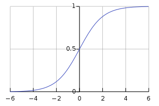
A sigmoid function is a bounded, differentiable, real function that is defined for all real input values and has a non-negative derivative at each point[1] and exactly one inflection point. A sigmoid "function" and a sigmoid "curve" refer to the same object.

In general, a sigmoid function is monotonic, and has a first derivative which is bell shaped. Conversely, the integral of any continuous, non-negative, bell-shaped function (with one local maximum and no local minimum, unless degenerate) will be sigmoidal. Thus the cumulative distribution functions for many common probability distributions are sigmoidal. One such example is the error function, which is related to the cumulative distribution function of a normal distribution.

A sigmoid function is constrained by a pair of horizontal asymptotes as ${\displaystyle x\rightarrow \pm \infty }$.

A sigmoid function is convex for values less than 0, and it is concave for values greater than 0.

Some sigmoid functions compared. In the drawing all functions are normalized in such a way that their slope at the origin is 1.

• Logistic function

${\displaystyle f(x)={\frac {1}{1+e^{-x}}}}$

• Hyperbolic tangent (shifted and scaled version of the logistic function, above)

${\displaystyle f(x)=\tanh x={\frac {e^{x}-e^{-x}}{e^{x}+e^{-x}}}}$

• Arctangent function

${\displaystyle f(x)=\arctan x}$

• Gudermannian function

${\displaystyle f(x)=\operatorname {gd} (x)=\int _{0}^{x}{\frac {1}{\cosh t}}\,dt=2\arctan \left(\tanh \left({\frac {x}{2}}\right)\right)}$

• Error function

${\displaystyle f(x)=\operatorname {erf} (x)={\frac {2}{\sqrt {\pi }}}\int _{0}^{x}e^{-t^{2}}\,dt}$

• Generalised logistic function

${\displaystyle f(x)=(1+e^{-x})^{-\alpha },\quad \alpha >0}$

• Smoothstep function

${\displaystyle f(x)={\begin{cases}\displaystyle {\left(\int _{0}^{1}(1-u^{2})^{N}\ du\right)^{-1}\int _{0}^{x}(1-u^{2})^{N}\ du},&|x|\leq 1\\\\\operatorname {sgn}(x)&|x|\geq 1\\\end{cases}}\,\quad N\geq 1}$

• Some algebraic functions, for example

${\displaystyle f(x)={\frac {x}{\sqrt {1+x^{2}}}}}$

Inverted logistic S-curve to model the relation between wheat yield and soil salinity. [2]

Many natural processes, such as those of complex system learning curves, exhibit a progression from small beginnings that accelerates and approaches a climax over time. When a specific mathematical model is lacking, a sigmoid function is often used.[3]

The van Genuchten–Gupta model is based on an inverted S-curve and applied to the response of crop yield to soil salinity.

Examples of the application of the logistic S-curve to the response of crop yield (wheat) to both the soil salinity and depth to water table in the soil are shown in logistic function#In agriculture: modeling crop response.

In artificial neural networks, sometimes non-smooth functions are used instead for efficiency; these are known as hard sigmoids.

In audio signal processing, sigmoid functions are used as waveshaper transfer functions to emulate the sound of analog circuitry clipping.[4]

In biochemistry and pharmacology, the Hill equation and Hill-Langmuir equation are sigmoid functions.

In computer graphics, and real-time rendering, some of the sigmoid functions are used to blend colors or geometry, between two values smoothly and without visible seams or discontinuities.

• Mitchell, Tom M. (1997). Machine Learning. WCB–McGraw–Hill. ISBN 978-0-07-042807-2.. In particular see "Chapter 4: Artificial Neural Networks" (in particular pp. 96–97) where Mitchell uses the word "logistic function" and the "sigmoid function" synonymously – this function he also calls the "squashing function" – and the sigmoid (aka logistic) function is used to compress the outputs of the "neurons" in multi-layer neural nets.
• Humphrys, Mark. "Continuous output, the sigmoid function". Properties of the sigmoid, including how it can shift along axes and how its domain may be transformed.

References

- Han, Jun; Morag, Claudio (1995). "The influence of the sigmoid function parameters on the speed of backpropagation learning". In Mira, José; Sandoval, Francisco (eds.). From Natural to Artificial Neural Computation. Lecture Notes in Computer Science. 930. pp. 195–201. doi:10.1007/3-540-59497-3_175. ISBN 978-3-540-59497-0.
- Software to fit an S-curve to a data set
- Gibbs, M.N. (Nov 2000). "Variational Gaussian process classifiers". IEEE Transactions on Neural Networks. 11 (6): 1458–1464. doi:10.1109/72.883477. PMID 18249869.
- Smith, Julius O. (2010). Physical Audio Signal Processing (2010 ed.). W3K Publishing. ISBN 978-0-9745607-2-4. Retrieved 28 March 2020.