Seconds pendulum
A seconds pendulum is a pendulum whose period is precisely two seconds; one second for a swing in one direction and one second for the return swing, a frequency of 1/2 Hz. A pendulum is a weight suspended from a pivot so that it can swing freely.[1] When a pendulum is displaced sideways from its resting equilibrium position, it is subject to a restoring force due to gravity that will accelerate it back toward the equilibrium position. When released, the restoring force combined with the pendulum's mass causes it to oscillate about the equilibrium position, swinging back and forth. The time for one complete cycle, a left swing and a right swing, is called the period. The period depends on the length of the pendulum, and also to a slight degree on its weight distribution (the moment of inertia about its own center of mass) and the amplitude (width) of the pendulum's swing.
Seconds pendulum and timekeeping
Time in physics is defined by its measurement: time is what a clock reads.[2] In classical, non-relativistic physics it is a scalar quantity and, like length, mass, and charge, is usually described as a fundamental quantity. Time can be combined mathematically with other physical quantities to derive other concepts such as motion, kinetic energy and time-dependent fields. Timekeeping is a complex of technological and scientific issues, and part of the foundation of recordkeeping.
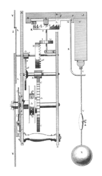
The pendulum clock was invented in 1656 by Dutch scientist and inventor Christiaan Huygens, and patented the following year. Huygens contracted the construction of his clock designs to clockmaker Salomon Coster, who actually built the clock. Huygens was inspired by investigations of pendulums by Galileo Galilei beginning around 1602. Galileo discovered the key property that makes pendulums useful timekeepers: isochronism, which means that the period of swing of a pendulum is approximately the same for different sized swings.[3][4] Galileo had the idea for a pendulum clock in 1637, which was partly constructed by his son in 1649, but neither lived to finish it.[5] The introduction of the pendulum, the first harmonic oscillator used in timekeeping, increased the accuracy of clocks enormously, from about 15 minutes per day to 15 seconds per day[6] leading to their rapid spread as existing 'verge and foliot' clocks were retrofitted with pendulums.
These early clocks, due to their verge escapements, had wide pendulum swings of 80–100°. In his 1673 analysis of pendulums, Horologium Oscillatorium, Huygens showed that wide swings made the pendulum inaccurate, causing its period, and thus the rate of the clock, to vary with unavoidable variations in the driving force provided by the movement. Clockmakers' realisation that only pendulums with small swings of a few degrees are isochronous motivated the invention of the anchor escapement around 1670, which reduced the pendulum's swing to 4–6°.[7] The anchor became the standard escapement used in pendulum clocks. In addition to increased accuracy, the anchor's narrow pendulum swing allowed the clock's case to accommodate longer, slower pendulums, which needed less power and caused less wear on the movement. The seconds pendulum (also called the Royal pendulum), 0.994 m (39.1 in) long, in which each swing takes one second, became widely used in quality clocks. The long narrow clocks built around these pendulums, first made by William Clement around 1680, became known as grandfather clocks. The increased accuracy resulting from these developments caused the minute hand, previously rare, to be added to clock faces beginning around 1690.[8]
The 18th and 19th century wave of horological innovation that followed the invention of the pendulum brought many improvements to pendulum clocks. The deadbeat escapement invented in 1675 by Richard Towneley and popularised by George Graham around 1715 in his precision "regulator" clocks gradually replaced the anchor escapement[9] and is now used in most modern pendulum clocks. Observation that pendulum clocks slowed down in summer brought the realisation that thermal expansion and contraction of the pendulum rod with changes in temperature was a source of error. This was solved by the invention of temperature-compensated pendulums; the mercury pendulum by George Graham in 1721 and the gridiron pendulum by John Harrison in 1726.[10] With these improvements, by the mid-18th century precision pendulum clocks achieved accuracies of a few seconds per week.
At the time the second was defined as a fraction of the Earth's rotation time or mean solar day and determined by clocks whose precision was checked by astronomical observations.[11][12] Solar time is a calculation of the passage of time based on the position of the Sun in the sky. The fundamental unit of solar time is the day. Two types of solar time are apparent solar time (sundial time) and mean solar time (clock time).
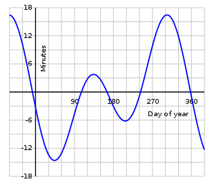
Mean solar time is the hour angle of the mean Sun plus 12 hours. This 12 hour offset comes from the decision to make each day start at midnight for civil purposes whereas the hour angle or the mean sun is measured from the zenith (noon).[13] The duration of daylight varies during the year but the length of a mean solar day is nearly constant, unlike that of an apparent solar day.[14] An apparent solar day can be 20 seconds shorter or 30 seconds longer than a mean solar day.[15] Long or short days occur in succession, so the difference builds up until mean time is ahead of apparent time by about 14 minutes near February 6 and behind apparent time by about 16 minutes near November 3. The equation of time is this difference, which is cyclical and does not accumulate from year to year.
Mean time follows the mean sun. Jean Meeus describes the mean sun as follows:
Consider a first fictitious Sun travelling along the ecliptic with a constant speed and coinciding with the true sun at the perigee and apogee (when the Earth is in perihelion and aphelion, respectively). Then consider a second fictitious Sun travelling along the celestial equator at a constant speed and coinciding with the first fictitious Sun at the equinoxes. This second fictitious sun is the mean Sun..."[16]
In 1936 French and German astronomers found that Earth rotation's speed is irregular. Since 1967 atomic clocks define the second.[17][Note 1]
Seconds pendulum and metrology
The length of a seconds pendulum was determined (in toises) by Marin Mersenne in 1644. In 1660, the Royal Society proposed that it be the standard unit of length. In 1671 Jean Picard measured this length at the Paris observatory. He found the value of 440.5 lines of the Toise of Châtelet which had been recently renewed. He proposed a universal toise (French: Toise universelle) which was twice the length of the seconds pendulum.[18][19] However, it was soon discovered that the length of a seconds pendulum varies from place to place: French astronomer Jean Richer had measured the 0.3% difference in length between Cayenne (in French Guiana) and Paris.[20]
Seconds pendulum and the figure of the Earth
Jean Richer and Giovanni Domenico Cassini measured the parallax of Mars between Paris and Cayenne in French Guiana when Mars was at its closest to Earth in 1672. They arrived at a figure for the solar parallax of 91/2 inches, equivalent to an Earth–Sun distance of about 22000 Earth radii. They were also the first astronomers to have access to an accurate and reliable value for the radius of Earth, which had been measured by their colleague Jean Picard in 1669 as 3269 thousand toises. Picard's geodetic observations had been confined to the determination of the magnitude of the earth considered as a sphere, but the discovery made by Jean Richer turned the attention of mathematicians to its deviation from a spherical form. The determination of the figure of the earth became a problem of the highest importance in astronomy, inasmuch as the diameter of the earth was the unit to which all celestial distances had to be referred.[21][22][23][24][11][25]
British physicist Isaac Newton, who used Picard's Earth measurement for establishing his law of universal gravity,[26] explained this variation of the seconds pendulum's length in his Principia Mathematica (1687) in which he outlined his theory and calculations on the shape of the Earth. Newton theorized correctly that the Earth was not precisely a sphere but had an oblate ellipsoidal shape, slightly flattened at the poles due to the centrifugal force of its rotation. Since the surface of the Earth is closer to its center at the poles than at the equator, gravity is stronger there. Using geometric calculations, he gave a concrete argument as to the hypothetical ellipsoid shape of the Earth.[27]
The goal of Principia was not to provide exact answer for natural phenomena, but to theorize potential solutions to these unresolved factors in science. Newton pushed for scientists to look further into the unexplained variables. Two prominent researchers that he inspired were Alexis Clairaut and Pierre Louis Maupertuis. They both sought to prove the validity of Newton's theory on the shape of the Earth. In order to do so, they went on an expedition to Lapland in an attempt to accurately measure the meridian arc. From such measurements they could calculate the eccentricity of the Earth, its degree of departure from a perfect sphere. Clairaut confirmed that Newton's theory that the Earth was ellipsoidal was correct, but his calculations were in error, and wrote a letter to the Royal Society of London with his findings.[28] The society published an article in Philosophical Transactions the following year in 1737 that revealed his discovery. Clairaut showed how Newton's equations were incorrect, and did not prove an ellipsoid shape to the Earth.[29] However, he corrected problems with the theory, that in effect would prove Newton's theory correct. Clairaut believed that Newton had reasons for choosing the shape that he did, but he did not support it in Principia. Clairaut's article did not provide a valid equation to back up his argument neither. This created much controversy in the scientific community.
It was not until Clairaut wrote Théorie de la figure de la terre in 1743 that a proper answer was provided. In it, he promulgated what is more formally known today as Clairaut's theorem. By applying Clairaut's theorem, Laplace found from 15 gravity values that the flattening of the Earth was 1/330. A modern estimate is 1/298.25642.[30]
In 1790, one year before the metre was ultimately based on a quadrant of the Earth, Talleyrand proposed that the metre be the length of the seconds pendulum at a latitude of 45°.[1] This option, with one-third of this length defining the foot, was also considered by Thomas Jefferson and others for redefining the yard in the United States shortly after gaining independence from the British Crown.[31]
Instead of the seconds pendulum method, the commission of the French Academy of Sciences – whose members included Lagrange, Laplace, Monge and Condorcet – decided that the new measure should be equal to one ten-millionth of the distance from the North Pole to the Equator (the quadrant of the Earth's circumference), measured along the meridian passing through Paris. Apart from the obvious consideration of safe access for French surveyors, the Paris meridian was also a sound choice for scientific reasons: a portion of the quadrant from Dunkirk to Barcelona (about 1000 km, or one-tenth of the total) could be surveyed with start- and end-points at sea level, and that portion was roughly in the middle of the quadrant, where the effects of the Earth's oblateness were expected to be the largest. The Spanish-French geodetic mission combined with an earlier mesurement of the Paris meridian arc and the Lapland geodetic mission had confirmed that the Earth was an oblate spheroid.[25] Moreover observations were made with a pendulum to determine the local acceleration due to local gravity and centrifugal acceleration; and these observations coincided with the geodetic results in proving that the Earth is flattened at the poles. The acceleration of a body near the surface of the Earth, which is measured with the seconds pendulum, is due to the combined effects of local gravity and centrifugal acceleration. The gravity diminishes with the distance from the center of the Earth while the centrifugal force augments with the distance from the axis of the Earth's rotation, it follows that the resulting acceleration towards the ground is 0.5% greater at the poles than at the Equator and that the polar diameter of the Earth is smaller than its equatorial diameter.[25][32][33][34][Note 2]
The Academy of Sciences planned to infer the flattening of the Earth from the length's differences between meridional portions corresponding to one degree of latitude. Pierre Méchain and Jean-Baptiste Delambre combined their measurements with the results of the Spanish-French geodetic mission and found a value of 1/334 for the Earth's flattening,[35] and they then extrapolated from their measurement of the Paris meridian arc between Dunkirk and Barcelona the distance from the North Pole to the Equator which was 5 130 740 toises. As the metre had to be equal to one ten-millionth of this distance, it was defined as 0.513074 toise or 3 feet and 11.296 lines of the Toise of Peru.[36] The Toise of Peru had been constructed in 1735 as the standard of reference in the Spanish-French Geodesic Mission, conducted in actual Ecuador from 1735 to 1744.[37]
Jean-Baptiste Biot and François Arago published in 1821 their observations completing those of Delambre and Mechain. It was an account of the length's variation of the degrees of latitude along the Paris meridian as well as the account of the variation of the seconds pendulum's length along the same meridian between Shetland and the Baleares. The seconds pendulum's length is a mean to measure g, the local acceleration due to local gravity and centrifugal acceleration, which varies depending on one's position on Earth (see Earth's gravity).[38][39][40]
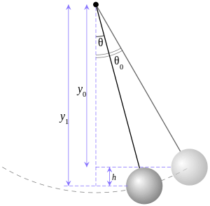
A simple pendulum is an example of harmonic oscillator:
Assuming no damping, the differential equation governing a simple pendulum of length , where is the local acceleration due to local gravity and centrifugal acceleration, is


If the maximal displacement of the pendulum is small, we can use the approximation and instead consider the equation


The solution to this equation is given by

where is the largest angle attained by the pendulum. The period, the time for one complete oscillation, is given by the expression


which is a good approximation of the actual period when is small.
The length of the seconds pendulum is a function of the time lapse of half a cycle


Being therefore .


The task of surveying the Paris meridian arc took more than six years (1792–1798). The technical difficulties were not the only problems the surveyors had to face in the convulsed period of the aftermath of the Revolution: Méchain and Delambre, and later Arago, were imprisoned several times during their surveys, and Méchain died in 1804 of yellow fever, which he contracted while trying to improve his original results in northern Spain. In the meantime, the commission of the French Academy of Sciences calculated a provisional value from older surveys of 443.44 lignes. This value was set by legislation on 7 April 1795.[41] While Méchain and Delambre were completing their survey, the commission had ordered a series of platinum bars to be made based on the provisional metre. When the final result was known, the bar whose length was closest to the meridional definition of the metre was selected and placed in the National Archives on 22 June 1799 (4 messidor An VII in the Republican calendar) as a permanent record of the result.[42] This standard metre bar became known as the Committee metre (French : Mètre des Archives).
Standards in the United States and U.S. Survey of the Coast
The Articles of Confederation, ratified by the colonies in 1781, contained the clause, "The United States in Congress assembled shall also have the sole and exclusive right and power of regulating the alloy and value of coin struck by their own authority, or by that of the respective states—fixing the standards of weights and measures throughout the United States". Article 1, section 8, of the Constitution of the United States (1789), transferred this power to Congress; "The Congress shall have power...To coin money, regulate the value thereof, and of foreign coin, and fix the standard of weights and measures".
In January 1790, President George Washington, in his first annual message to Congress stated that, "Uniformity in the currency, weights, and measures of the United States is an object of great importance, and will, I am persuaded, be duly attended to", and ordered Secretary of State Thomas Jefferson to prepare a plan for Establishing Uniformity in the Coinage, Weights, and Measures of the United States, afterwards referred to as the Jefferson report. On October 25, 1791, Washington appealed a third time to Congress, "A uniformity of the weights and measures of the country is among the important objects submitted to you by the Constitution and if it can be derived from a standard at once invariable and universal, must be no less honorable to the public council than conducive to the public convenience".
The original predecessor agency of the National Geodetic Survey was the United States Survey of the Coast, created within the United States Department of the Treasury by an Act of Congress on February 10, 1807, to conduct a "Survey of the Coast."[43][44] The Survey of the Coast, the United States government's first scientific agency,[44] represented the interest of the administration of President Thomas Jefferson in science and the stimulation of international trade by using scientific surveying methods to chart the waters of the United States and make them safe for navigation. A Swiss immigrant with expertise in both surveying and the standardisation of weights and measures, Ferdinand R. Hassler, was selected to lead the Survey.[45]
Hassler submitted a plan for the survey work involving the use of triangulation to ensure scientific accuracy of surveys, but international relations prevented the new Survey of the Coast from beginning its work; the Embargo Act of 1807 brought American overseas trade virtually to a halt only a month after Hassler's appointment and remained in effect until Jefferson left office in March 1809. It was not until 1811 that Jefferson's successor, President James Madison, sent Hassler to Europe to purchase the instruments necessary to conduct the planned survey, as well as standardised weights and measures. Hassler departed on August 29, 1811, but eight months later, while he was in England, the War of 1812 broke out, forcing him to remain in Europe until its conclusion in 1815. Hassler did not return to the United States until August 16, 1815.[45]
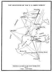
The Survey finally began surveying operations in 1816, when Hassler started work in the vicinity of New York City. Preliminary baselines' measurements were undertaken in 1817. The first baseline was measured in 1834 and verified in 1844 and 1857.[45][46][47] The unit of length to which all distances measured in the U. S. coast survey would be referred was the Committee metre (French: Mètre des Archives), of which Ferdinand Rudolph Hassler had brougth a copy in the United States in 1805.[48][49]
In 1821, John Quincy Adams had declared "Weights and measures may be ranked among the necessities of life to every individual of human society".[50] From 1830 until 1901, the role of overseeing weights and measures was carried out by the Office of Standard Weights and Measures, which was part of the United States Department of the Treasury.[51] Ferdinand Rudolph Hassler became the head of the Bureau of Weights and Measures in the Treasury Department where he carried out the early work of establishing the standards of weights and measures in the United States, with the involvement of fellow Swiss immigrant Albert Gallatin, who in 1827 brought from Europe a troy pound of brass which was made the standard of mass in 1828. Hassler undertook a complete investigation of the national standards in 1830, but it was not until 1838, that a uniform set of standards was worked out.
The International Geodetic Association: a new era in the science of geodesy
In 1835, the invention of the telegraph by Samuel Morse allowed new progresses in the field of geodesy as longitudes were determined with greater accuracy.[35] Moreover the publication in 1838 of Friedrich Wilhelm Bessel’s Gradmessung in Ostpreussen marked a new era in the science of geodesy. Here was found the method of least squares applied to the calculation of a network of triangles and the reduction of the observations generally. The systematic manner in which all the observations were taken with the view of securing final results of extreme accuracy was admirable.[25] Bessel was also the first scientist who realised the effect later called personal equation, that several simultaneously observing persons determine slightly different values, especially recording the transition time of stars.[52] For his survey Bessel used a copy of the Toise of Peru constructed in 1823 by Fortin in Paris.[37]
The first clear and concise exposition of the method of least squares was published by Legendre in 1805.[53] The technique is described as an algebraic procedure for fitting linear equations to data and Legendre demonstrates the new method by analyzing the same data as Laplace for the shape of the earth. The value of Legendre's method of least squares was immediately recognised by leading astronomers and geodesists of the time.
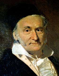
In 1809 Carl Friedrich Gauss published his method of calculating the orbits of celestial bodies. In that work he claimed to have been in possession of the method of least squares since 1795. This naturally led to a priority dispute with Legendre. However, to Gauss's credit, he went beyond Legendre and succeeded in connecting the method of least squares with the principles of probability and to the normal distribution. He had managed to complete Laplace's program of specifying a mathematical form of the probability density for the observations, depending on a finite number of unknown parameters, and define a method of estimation that minimises the error of estimation. Gauss showed that the arithmetic mean is indeed the best estimate of the location parameter by changing both the probability density and the method of estimation. He then turned the problem around by asking what form the density should have and what method of estimation should be used to get the arithmetic mean as estimate of the location parameter. In this attempt, he invented the normal distribution.
An early demonstration of the strength of Gauss' method came when it was used to predict the future location of the newly discovered asteroid Ceres. On 1 January 1801, the Italian astronomer Giuseppe Piazzi discovered Ceres and was able to track its path for 40 days before it was lost in the glare of the sun. Based on these data, astronomers desired to determine the location of Ceres after it emerged from behind the sun without solving Kepler's complicated nonlinear equations of planetary motion. The only predictions that successfully allowed Hungarian astronomer Franz Xaver von Zach to relocate Ceres were those performed by the 24-year-old Gauss using least-squares analysis.
In 1810, after reading Gauss's work, Laplace, after proving the central limit theorem, used it to give a large sample justification for the method of least squares and the normal distribution. In 1822, Gauss was able to state that the least-squares approach to regression analysis is optimal in the sense that in a linear model where the errors have a mean of zero, are uncorrelated, and have equal variances, the best linear unbiased estimator of the coefficients is the least-squares estimator. This result is known as the Gauss–Markov theorem.
The idea of least-squares analysis was also independently formulated by the American Robert Adrain in 1808. In the next two centuries workers in the theory of errors and in statistics found many different ways of implementing least squares.[54]

In 1860, the Russian Government at the instance of Otto Wilhelm von Struve invited the Governments of Belgium, France, Prussia and England to connect their triangulations in order to measure the length of an arc of parallel in latitude 52° and to test the accuracy of the figure and dimensions of the Earth, as derived from the measurements of arc of meridian. In order to combine the measurements it was necessary to compare the geodetic standards of length used in the different countries.The British Government invited those of France, Belgium, Prussia, Russia, India, Australia, Austria, Spain, United States and Cape of Good Hope to send their standards to the Ordnance Survey office in Southampton. Notably the geodetic standards of France, Spain and United States were based on the metric system, whereas those of Prussia, Belgium and Russia where calibrated against the toise, of which the oldest physical representative was the Toise of Peru.[48][37]
In 1861 Johann Jacob Baeyer published a report suggesting that European countries should cooperate in the determination of the figure of the Earth. In 1862, when Denmark, Saxe-Gotha, the Netherlands, Russia (for Poland), Switzerland, Baden, Saxony, Italy, Austria, Sweden, Norway, Bavaria, Mecklenburg, Hanover and Belgium decided to participate, Bessel's Toise was adopted as international geodetic standard.[55]
The Congress of 1866 made use of the metric system in commerce a legally protected activity through the passage of Metric Act of 1866.[56]
In 1867 besides Russia and Portugal, Spain joined the geodetic association and was represented by Carlos Ibáñez e Ibáñez de Ibero. He had devised a geodetic standard calibrated against the metre which had been compared to the Toise of Borda, the copy of the Toise of Peru constructed for the measurement of the Paris meridian arc by Delambre and Mechain. Copies of the Spanish metric geodetic standard were made for some of the great European countries and for Egypt. The European geodetic association (German: Europäische Gradmessung) at its Second General Conference in 1867 called for the creation of a new, international prototype metre (IPM) and the arrangement of a system where national standards could be compared with it. The international prototype would also be a "line standard"; that is, the metre was defined as the distance between two lines marked on the bar, so avoiding the wear problems of end standards.
The French government gave practical support to the creation of an International Metre Commission, which met in Paris in 1870 and again in 1872 with the participation of about thirty countries.
Fondator of the Spanish Geographic Institute, Carlos Ibáñez e Ibáñez de Ibero had collaborated with the French since 1853 on the completion of the West Europe-Africa Meridian-arc (French: Meridienne de France), which would then extend from Shetland to the Sahara, by expanding the continental geodetic survey in Spain and by connecting Spanish and Algerian geodetic network over the Mediterranean sea.
As a forerunner in Europe, Spain had adopted the metre as geodetic standard, contributed to the Europäische Gradmessung's decision to adopt the metre and played a leading role in the fondation of the International Bureau of Weights and Measures. Indeed Carlos Ibáñez e Ibáñez de Ibero took part in the Committee of preparatory research from the first meeting of the International Metre Commission in 1870, became president of the permanent Committee of the International Metre Commission in 1872, represented Spain at the 1875 conference of the Metre Convention and at the first General Conference on Weights and Measures in 1889 and was the first president of the International Committee for Weights and Measures from 1875 to 1891.[57][58]
On May 20, 1875, 17 out of 20 countries signed a document known as the Metric Convention or the Treaty of the Metre, which established the International Bureau of Weights and Measures under the control of an international committee elected by the General Conference on Weights and Measures.[56]
Charles Sanders Pierce was instructed early in the spring of 1875 to proceed to Europe for the purpose of making pendulum experiments to chief initial stations for operations of this sort, in order to bring the determinations of the forces of gravity in America into communication with those of other parts of the world; and also for the purpose of making a careful study of the methods of pursuing these researches in the different countries of Europe.[59]
In 1877 Charles S. Pierce attended the 5th General conference of the Europäische Gradmessung in Stuttgart where he exposed his work on seconds pendulum and expressed his concern about the accuracy of gravity measurement.[60] In 1880 the French Academy of sciences adopted Pierce's measurement of the seconds pendulum length in Paris, which was 993.934 millimetres.[32]
In 1886 the association of geodesy changed name for the International Geodetic Association, which Carlos Ibáñez e Ibáñez de Ibero presided up to his death in 1891. During this period the International Geodetic Association (German: Internationale Erdmessung) gained worldwide importance with the joining of United States, Mexico, Chile, Argentina and Japan.[61][62][57]
In 1901, in response to a bill proposed by Congressman James H. Southard (R, Ohio), the National Bureau of Standards was founded with the mandate to provide standard weights and measures, and to serve as the national physical laboratory for the United States. (Southard had previously sponsored a bill for metric conversion of the United States.)[63] President Theodore Roosevelt appointed Samuel W. Stratton as the first director. The budget for the first year of operation was $40,000. The Bureau took custody of the copies of the kilogram and metre bars that were the standards for US measures, and set up a program to provide metrology services for United States scientific and commercial users.
Efforts to supplement the various national surveying systems, which begun in the 19th century with the foundation of the Mitteleuropäische Gradmessung, resulted in a series of global ellipsoids of the Earth (e.g., Helmert 1906, Hayford 1910/ 1924) which would later lead to develop the World Geodetic System.
Standard gravity and the international prototype metre
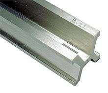
The construction of the international prototype metre and the copies which would be national standards was at the limits of the technology of the time. The bars were to be made of a special alloy, 90% platinum and 10% iridium, which is significantly harder than pure platinum, and have a special X-shaped cross section (a "Tresca section", named after French engineer Henri Tresca) to minimise the effects of torsional strain during length comparisons.[64] The first castings proved unsatisfactory, and the job was given to the London firm of Johnson Matthey who succeeded in producing thirty bars to the required specification. One of these, No. 6, was determined to be identical in length to the mètre des Archives, and was consecrated as the international prototype metre at the first meeting of the CGPM in 1889. The other bars, duly calibrated against the international prototype, were distributed to the signatory nations of the Metre Convention for use as national standards.[65] For example, the United States received No. 27 with a calibrated length of 0.999 9984 m ± 0.2 µm (1.6 µm short of the international prototype).[66]
The first (and only) follow-up comparison of the national standards with the international prototype was carried out between 1921 and 1936,[64][65] and indicated that the definition of the metre was preserved to within 0.2 µm.[67] At this time, it was decided that a more formal definition of the metre was required (the 1889 decision had said merely that the "prototype, at the temperature of melting ice, shall henceforth represent the metric unit of length"), and this was agreed at the 7th CGPM in 1927.[68]
The unit of length is the metre, defined by the distance, at 0°, between the axes of the two central lines marked on the bar of platinum–iridium kept at the Bureau International des Poids et Mesures and declared Prototype of the metre by the 1st Conférence Générale des Poids et Mesures, this bar being subject to standard atmospheric pressure and supported on two cylinders of at least one centimetre diameter, symmetrically placed in the same horizontal plane at a distance of 571 mm from each other.
Already in the early days of its existence, the International Committee for Weights and Measures (CIPM) proceeded to define a standard thermometric scale, using the boiling point of water. Since the boiling point varies with the atmospheric pressure, the CIPM needed to define a standard atmospheric pressure. The definition they chose was based on the weight of a column of mercury of 760 mm. But since that weight depends on the local gravity, they now also needed a standard gravity. The 1887 CIPM meeting decided as follows:
The value of this standard acceleration due to gravity is equal to the acceleration due to gravity at the International Bureau (alongside the Pavillon de Breteuil) divided by 1.0003322, the theoretical coefficient required to convert to a latitude of 45° at sea level.[69]
All that was needed to obtain a numerical value for standard gravity was now to measure the gravitational strength at the International Bureau. This task was given to Gilbert Étienne Defforges of the Geographic Service of the French Army. The value he found, based on measurements taken in March and April 1888, was 9.80991(5) m⋅s−2.[70]
This result formed the basis for determining the value still used today for standard gravity. The third General Conference on Weights and Measures, held in 1901, adopted a resolution declaring as follows:
The value adopted in the International Service of Weights and Measures for the standard acceleration due to Earth's gravity is 980.665 cm/s2, value already stated in the laws of some countries.[71]
The numeric value adopted for ɡ0 was, in accordance with the 1887 CIPM declaration, obtained by dividing Defforges's result – 980.991 cm⋅s−2 in the cgs system then en vogue – by 1.0003322 while not taking more digits than warranted considering the uncertainty in the result.
See also
Notes
- ↑ For further informations see atomic time.
- ↑ Gravity diminishes proportionally to the square of the distance from the center of the Earth. Centrifugal force is a pseudo force corresponding to inertia and is related to the speed of rotation of an object situated at the surface of the Earth, which is proportional to the distance from the axis of the Earth's rotation: v = 2πR/T.
References
- 1 2 Seconds pendulum
- ↑ Considine, Douglas M.; Considine, Glenn D. (1985). Process instruments and controls handbook (3 ed.). McGraw-Hill. pp. 18–61. ISBN 0-07-012436-1.
- ↑ "Huygens' Clocks". Stories. Science Museum, London, UK. Retrieved 2007-11-14.
- ↑ "Pendulum Clock". The Galileo Project. Rice Univ. Retrieved 2007-12-03.
- ↑ A modern reconstruction can be seen at "Pendulum clock designed by Galileo, Item #1883-29". Time Measurement. Science Museum, London, UK. Retrieved 2007-11-14.
- ↑ Bennet, Matthew; et al. (2002). "Huygens' Clocks" (PDF). Georgia Institute of Technology. Archived from the original (PDF) on 2008-04-10. Retrieved 2007-12-04. , p.3, also published in Proceedings of the Royal Society of London, A 458, 563–579
- ↑ Headrick, Michael (2002). "Origin and Evolution of the Anchor Clock Escapement". Control Systems magazine. Inst. of Electrical and Electronic Engineers. 22 (2). Archived from the original on October 26, 2009. Retrieved 2007-06-06.
- ↑ Milham 1945, p. 190
- ↑ Milham 1945, p.181, 441
- ↑ Milham 1945, pp. 193–195
- 1 2 texte, Picard, Jean (1620-1682). Auteur du (1671). "Mesure de la terre [par l'abbé Picard]". Gallica. p. 4. Retrieved 2018-09-28.
- ↑ Alain Bernard (2018-04-15), Le système solaire 2 : La révolution de la Terre, retrieved 2018-10-12
- ↑ "Archived copy" (PDF). Archived (PDF) from the original on 2018-03-28. Retrieved 2018-03-28.
- ↑ For a discussion of the slight changes that affect the mean solar day, see the ΔT article.
- ↑ "The duration of the true solar day" Archived 2009-08-26 at the Wayback Machine.. Pierpaolo Ricci. pierpaoloricci.it. (Italy)
- ↑ Meeus, J. (1998). Astronomical Algorithms. 2nd ed. Richmond VA: Willmann-Bell. p. 183.
- ↑ "Revivre notre histoire | Les 350 ans de l'Observatoire de Paris". 350ans.obspm.fr (in French). Retrieved 2018-09-28.
- ↑ texte, Picard, Jean (1620-1682). Auteur du (1671). "Mesure de la terre [par l'abbé Picard]". Gallica. pp. 3–4. Retrieved 2018-09-13.
- ↑ Bigourdan, Guillaume (1901). Le système métrique des poids et mesures ; son établissement et sa propagation graduelle, avec l'histoire des opérations qui ont servi à déterminer le mètre et le kilogramme. University of Ottawa. Paris : Gauthier-Villars. pp. 6–8.
- ↑ Poynting, John Henry; Thomson, Joseph John (1907). A Textbook of Physics. C. Griffin. p. 20.
- ↑ Bond, Peter; Dupont-Bloch, Nicolas (2014). L'exploration du système solaire (in French). Louvain-la-Neuve: De Boeck. pp. 5–6. ISBN 9782804184964.
- ↑ "Première détermination de la distance de la Terre au Soleil | Les 350 ans de l'Observatoire de Paris". 350ans.obspm.fr (in French). Retrieved 2018-10-02.
- ↑ "1967LAstr..81..234G Page 234". adsbit.harvard.edu. Retrieved 2018-10-02.
- ↑ "INRP - CLEA - Archives : Fascicule N° 137, Printemps 2012 Les distances". clea-astro.eu (in French). Retrieved 2018-10-02.
- 1 2 3 4 "Earth, Figure of the", 1911 Encyclopædia Britannica, Volume 8, retrieved 2018-10-02
- ↑ texte, Biot, Jean-Baptiste (1774-1862). Auteur du; texte, Arago, François (1786-1853). Auteur du (1821). "Recueil d'observations géodésiques, astronomiques et physiques, exécutées par ordre du Bureau des longitudes de France en Espagne, en France, en Angleterre et en Écosse, pour déterminer la variation de la pesanteur et des degrés terrestres sur le prolongement du méridien de Paris... rédigé par MM. Biot et Arago,..." Gallica. p. 523. Retrieved 2018-10-10.
- ↑ Newton, Isaac. Principia, Book III, Proposition XIX, Problem III.
- ↑ Greenburg, John (1995). The Problem of the Earth's Shape from Newton to Clairaut. New York: Cambridge University Press. p. 132. ISBN 0-521-38541-5.
- ↑ Clairaut, Alexis; Colson, John (1737). "An Inquiry concerning the Figure of Such Planets as Revolve about an Axis, Supposing the Density Continually to Vary, from the Centre towards the Surface". Philosophical Transactions. JSTOR 103921.
- ↑ Table 1.1 IERS Numerical Standards (2003))
- ↑ Cochrane, Rexmond (1966). "Appendix B: The metric system in the United States". Measures for progress: a history of the National Bureau of Standards. U.S. Department of Commerce. p. 532.
- 1 2 texte, Académie des sciences (France). Auteur du (1880). "Comptes rendus hebdomadaires des séances de l'Académie des sciences / publiés... par MM. les secrétaires perpétuels". Gallica. pp. 1463–1466. Retrieved 2018-10-10.
- ↑ Alain Bernard (2017-12-29), Le système solaire 1: la rotation de la Terre, retrieved 2018-10-12
- ↑ ...)., Cassidy, David C. (1945- (2014). Comprendre la physique. Holton, Gerald James, (1922- ...)., Rutherford, Floyd James, (1924- ...)., Faye, Vincent., Bréard, Sébastien. Lausanne: Presses polytechniques et universitaires romandes. pp. 173, 149. ISBN 9782889150830. OCLC 895784336.
- 1 2 Levallois, Jean-Jacques (May–June 1986). "L'Académie Royale des Sciences et la Figure de la Terre" [The Royal Academy of Sciences and the Shape of the Earth]. La Vie des sciences (in French). France: Académie des sciences: 290. Retrieved 2018-09-04 – via Gallica.
- ↑ "Histoire du mètre". Direction Générale des Entreprises (DGE) (in French). Retrieved 2018-09-28.
- 1 2 3 Clarke, Alexander Ross (1867-01-01). "X. Abstract of the results of the comparisons of the standards of length of England, France, Belgium, Prussia, Russia, India, Australia, made at the ordnance Survey Office, Southampton". Philosophical Transactions of the Royal Society of London. 157: 161–180. doi:10.1098/rstl.1867.0010. ISSN 0261-0523.
- ↑ Larousse, Pierre (1874). Larousse, Pierre, ed. (1874), "Métrique", Grand dictionnaire universel du XIXe siècle, 11. Paris. pp. 163–164.
- ↑ Paul., Murdin, (2009). Full meridian of glory : perilous adventures in the competition to measure the Earth. New York: Copernicus Books/Springer. ISBN 9780387755342. OCLC 314175913.
- ↑ texte, Biot, Jean-Baptiste (1774-1862). Auteur du; texte, Arago, François (1786-1853). Auteur du (1821). "Recueil d'observations géodésiques, astronomiques et physiques, exécutées par ordre du Bureau des longitudes de France en Espagne, en France, en Angleterre et en Écosse, pour déterminer la variation de la pesanteur et des degrés terrestres sur le prolongement du méridien de Paris... rédigé par MM. Biot et Arago,..." Gallica. Retrieved 2018-09-21.
- ↑ National Industrial Conference Board (1921). The metric versus the English system of weights and measures ... The Century Co. pp. 10–11. Retrieved 2011-04-05.
- ↑

- ↑ "Coast and Geodetic Survey Heritage - NOAA Central Library". 2015-12-19. Retrieved 2018-09-08.
- 1 2 "NOAA History - NOAA Legacy Timeline - 1800's". www.history.noaa.gov. Retrieved 2018-09-08.
- 1 2 3 "Access and Use - NOAA Central Library". 2014-09-06. Retrieved 2018-09-08.
- ↑ "The Coast Survey 1807-1867 - NOAA Central Library". 2015-09-25. Retrieved 2018-10-08.
- ↑ "NIST Special Publication 1068 Ferdinand Rudolph Hassler (1770-1843) A Twenty Year Retrospective, 1987-2007" (PDF). National Institute of Standards and Technology. March 2007. pp. 51–52. Archived from the original (PDF) on 28 November 2017. Retrieved 8 October 2018.
- 1 2 Clarke, Alexander Ross (1873). "XIII. Results of the comparisons of the standards of length of England, Austria, Spain, United States, Cape of Good Hope, and of a second Russian standard, made at the Ordnance Survey Office, Southampton. With a preface and notes on the Greek and Egyptian measures of length by Sir Henry James". Philosophical Transactions.
- ↑ "e-expo: Ferdinand Rudolf Hassler". www.f-r-hassler.ch. Retrieved 2018-09-08.
- ↑ NBS special publication 447 Archived October 17, 2011,at the "Wayback Machine", Wikipedia, 2018-09-20, retrieved 2018-09-24
- ↑ "Records of the National Institute of Standards and Technology". National Archives. 2016-08-15. Retrieved 2018-09-24.
- ↑ Hoffmann, Christoph (2007). "Constant differences: Friedrich Wilhelm Bessel, the concept of the observer in early nineteenth-century practical astronomy and the history of the personal equation". British Journal for the History of Science. 40 (3): 333–365. doi:10.1017/s0007087407009478.
- ↑ Legendre, Adrien-Marie (1805), Nouvelles méthodes pour la détermination des orbites des comètes [New Methods for the Determination of the Orbits of Comets] (in French), Paris: F. Didot
- ↑ Aldrich, J. (1998). "Doing Least Squares: Perspectives from Gauss and Yule". International Statistical Review. 66 (1): 61–81. doi:10.1111/j.1751-5823.1998.tb00406.x.
- ↑ "A Note on the History of the IAG". IAG Homepage. Retrieved 2018-09-30.
- 1 2 "Weights and Measures Standards of the United States a brief history" (PDF). ts.nist.gov. p. 41, 22. Archived from the original (PDF) on October 26, 2011. Retrieved 2011-09-28.
- 1 2 Soler, T. (1997-02-10). "A profile of General Carlos Ibáñez e Ibáñez de Ibero: first president of the International Geodetic Association". Journal of Geodesy. 71 (3): 176–188. doi:10.1007/s001900050086. ISSN 0949-7714.
- ↑ "BIPM - Presidents of the CIPM". www.bipm.org. Retrieved 2018-09-30.
- ↑ "Informe de Charles S. Peirce sobre su segundo viaje europeo para el informe anual del superintendente del U. S. Coast Survey 18.05.1877". www.unav.es. Retrieved 2018-10-10.
- ↑ "Quinta Conferencia Geodésica Internacional Association Géodésique Internationale o Europäischen Gradmessung Stuttgart, 27 de septiembre-2 de octubre de 1877". www.unav.es. Retrieved 2018-10-10.
- ↑ Torge, Wolfgang (2015), "From a Regional Project to an International Organization: The "Baeyer-Helmert-Era" of the International Association of Geodesy 1862–1916", International Association of Geodesy Symposia, Springer International Publishing, pp. 3–18, doi:10.1007/1345_2015_42, ISBN 9783319246031, retrieved 2018-10-02
- ↑ Torge, W. (2005-03-25). "The International Association of Geodesy 1862 to 1922: from a regional project to an international organization". Journal of Geodesy. 78 (9): 558–568. doi:10.1007/s00190-004-0423-0. ISSN 0949-7714.
- ↑ Perry, John (1953). The Story of Standards. Library of Congress Cat. No. 55-11094: Funk and Wagnalls. p. 123.
- 1 2 Nelson, Robert A. (December 1981). "Foundations of the international system of units (SI)" (PDF). The Physics Teacher: 596–613.
- 1 2 The BIPM and the evolution of the definition of the metre, International Bureau of Weights and Measures, retrieved 2016-08-30
- ↑ National Prototype Meter No. 27, National Institute of Standards and Technology, retrieved 2010-08-17
- ↑ Barrell, H. (1962). "The Metre". Contemporary Physics. 3 (6): 415–434. Bibcode:1962ConPh...3..415B. doi:10.1080/00107516208217499.
- ↑ International Bureau of Weights and Measures (2006), The International System of Units (SI) (PDF) (8th ed.), pp. 142–143, 148, ISBN 92-822-2213-6, archived (PDF) from the original on 2017-08-14
- ↑ Terry Quinn (2011). From Artefacts to Atoms: The BIPM and the Search for Ultimate Measurement Standards. Oxford University Press. p. 127. ISBN 978-0-19-530786-3.
- ↑ M. Amalvict (2010). "Chapter 12. Absolute gravimetry at BIPM, Sèvres (France), at the time of Dr. Akihiko Sakuma". In Stelios P. Mertikas. Gravity, Geoid and Earth Observation: IAG Commission 2: Gravity Field. Springer. pp. 84–85. ISBN 978-3-642-10634-7.
- ↑ "Resolution of the 3rd CGPM (1901)". BIPM. Retrieved July 19, 2015.