Linear form

In linear algebra, a linear functional or linear form (also called a one-form or covector) is a linear map from a vector space to its field of scalars. In ℝⁿ, if vectors are represented as column vectors, then linear functionals are represented as row vectors, and their action on vectors is given by the dot product, or the matrix product with the row vector on the left and the column vector on the right. In general, if V is a vector space over a field k, then a linear functional f is a function from V to k that is linear:

f(\vec{v}+\vec{w}) = f(\vec{v})+f(\vec{w})

for all

\vec{v}, \vec{w}\in V

f(a\vec{v}) = af(\vec{v})

for all

\vec{v}\in V, a\in k.

The set of all linear functionals from V to k, Hom_k(V,k), forms a vector space over k with the addition of the operations of addition and scalar multiplication (defined pointwise). This space is called the dual space of V, or sometimes the algebraic dual space, to distinguish it from the continuous dual space. It is often written V^∗, V′, or V^ᐯ when the field k is understood.

Continuous linear functionals

If V is a topological vector space, the space of continuous linear functionals — the continuous dual — is often simply called the dual space. If V is a Banach space, then so is its (continuous) dual. To distinguish the ordinary dual space from the continuous dual space, the former is sometimes called the algebraic dual space. In finite dimensions, every linear functional is continuous, so the continuous dual is the same as the algebraic dual, but in infinite dimensions the continuous dual is a proper subspace of the algebraic dual.

Examples and applications

Linear functionals in Rⁿ

Suppose that vectors in the real coordinate space Rⁿ are represented as column vectors

\vec{x} = \begin{bmatrix}x_1\\ \vdots\\ x_n\end{bmatrix}.

For each row vector [a₁ … a_n] there is a linear functional f defined by

f({\vec {x}})=a_{1}x_{1}+\cdots +a_{n}x_{n},

and each linear functional can be expressed in this form.

This can be interpreted as either the matrix product or the dot product of the row vector [a₁ ... a_n] and the column vector ${\vec {x}}$ :

f(\vec{x}) = [a_1 \dots a_n] \begin{bmatrix}x_1\\ \vdots\\ x_n\end{bmatrix}.

Integration

Linear functionals first appeared in functional analysis, the study of vector spaces of functions. A typical example of a linear functional is integration: the linear transformation defined by the Riemann integral

I(f) = \int_a^b f(x)\, dx

is a linear functional from the vector space C[a, b] of continuous functions on the interval [a, b] to the real numbers. The linearity of $I$ follows from the standard facts about the integral:

{\begin{aligned}I(f+g)&=\int _{a}^{b}[f(x)+g(x)]\,dx=\int _{a}^{b}f(x)\,dx+\int _{a}^{b}g(x)\,dx=I(f)+I(g)\\I(\alpha f)&=\int _{a}^{b}\alpha f(x)\,dx=\alpha \int _{a}^{b}f(x)\,dx=\alpha I(f).\end{aligned}}

Evaluation

Let P_n denote the vector space of real-valued polynomial functions of degree ≤n defined on an interval [a, b]. If c ∈ [a, b], then let ev_c : P_n → R be the evaluation functional

\operatorname{ev}_c f = f(c).

The mapping f → f(c) is linear since

{\begin{aligned}(f+g)(c)&=f(c)+g(c)\\(\alpha f)(c)&=\alpha f(c).\end{aligned}}

If x₀, ..., x_n are n + 1 distinct points in [a, b], then the evaluation functionals ev_{x_i}, i = 0, 1, ..., n form a basis of the dual space of P_n. (Lax (1996) proves this last fact using Lagrange interpolation.)

Application to quadrature

The integration functional $I$ defined above defines a linear functional on the subspace $P n$ of polynomials of degree $\leq n$ . If $x 0, ..., x n$ are $n + 1$ distinct points in $[a, b]$ , then there are coefficients $a 0, ..., a n$ for which

I(f) = a_0 f(x_0) + a_1 f(x_1) + \dots + a_n f(x_n)

for all $f \in P n$ . This forms the foundation of the theory of numerical quadrature.

This follows from the fact that the linear functionals $ev x i : f \to f (x i)$ defined above form a basis of the dual space of $P n$ .^[1]

Linear functionals in quantum mechanics

Linear functionals are particularly important in quantum mechanics. Quantum mechanical systems are represented by Hilbert spaces, which are anti–isomorphic to their own dual spaces. A state of a quantum mechanical system can be identified with a linear functional. For more information see bra–ket notation.

Distributions

In the theory of generalized functions, certain kinds of generalized functions called distributions can be realized as linear functionals on spaces of test functions.

Properties

Any linear functional L is either trivial (equal to 0 everywhere) or surjective onto the scalar field. Indeed, this follows since just as the image of a vector subspace under a linear transformation is a subspace, so is the image of V under L. however, the only subspaces (i.e., k-subspaces) of k are {0} and k itself.
A linear functional is continuous if and only if its kernel is closed. ^[2]
Linear functionals with the same kernel are proportional.
The absolute value of any linear functional is a seminorm on its vector space.

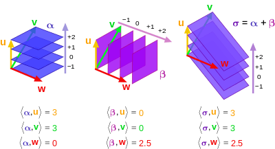
Visualizing linear functionals

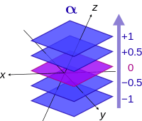
Geometric interpretation of a 1-form α as a stack of hyperplanes of constant value, each corresponding to those vectors that α maps to a given scalar value shown next to it along with the "sense" of increase. The zero plane is through the origin.

In finite dimensions, a linear functional can be visualized in terms of its level sets. In three dimensions, the level sets of a linear functional are a family of mutually parallel planes; in higher dimensions, they are parallel hyperplanes. This method of visualizing linear functionals is sometimes introduced in general relativity texts, such as Gravitation by Misner, Thorne & Wheeler (1973).

Dual vectors and bilinear forms

Linear functionals (1-forms) α, β and their sum σ and vectors u, v, w, in 3d Euclidean space. The number of (1-form) hyperplanes intersected by a vector equals the inner product.^[3]

Every non-degenerate bilinear form on a finite-dimensional vector space V induces an isomorphism V → V^∗ : v ↦ v^∗ such that

v^{*}(w):=\langle v,w\rangle \quad \forall w\in V,

where the bilinear form on V is denoted ⟨ , ⟩ (for instance, in Euclidean space ⟨v, w⟩ = v ⋅ w is the dot product of v and w).

The inverse isomorphism is V^∗ → V : v^∗ ↦ v, where v is the unique element of V such that

\langle v,w\rangle =v^{*}(w)\quad \forall w\in V.

The above defined vector v^∗ ∈ V^∗ is said to be the dual vector of v ∈ V.

In an infinite dimensional Hilbert space, analogous results hold by the Riesz representation theorem. There is a mapping V → V^∗ into the continuous dual space V^∗. However, this mapping is antilinear rather than linear.

Bases in finite dimensions

Basis of the dual space in finite dimensions

Let the vector space V have a basis $\vec{e}_1, \vec{e}_2,\dots,\vec{e}_n$ , not necessarily orthogonal. Then the dual space V* has a basis $\tilde{\omega}^1,\tilde{\omega}^2,\dots,\tilde{\omega}^n$ called the dual basis defined by the special property that

\tilde{\omega}^i (\vec e_j) = \left\{\begin{matrix} 1 &\mathrm{if}\ i=j\\ 0 &\mathrm{if}\ i\not=j.\end{matrix}\right.

Or, more succinctly,

\tilde{\omega}^i (\vec e_j) = \delta^i_j

where δ is the Kronecker delta. Here the superscripts of the basis functionals are not exponents but are instead contravariant indices.

A linear functional ${\tilde {u}}$ belonging to the dual space $\tilde{V}$ can be expressed as a linear combination of basis functionals, with coefficients ("components") u_i,

\tilde{u} = \sum_{i=1}^n u_i \, \tilde{\omega}^i.

Then, applying the functional ${\tilde {u}}$ to a basis vector e_j yields

{\tilde {u}}({\vec {e}}_{j})=\sum _{i=1}^{n}\left(u_{i}\,{\tilde {\omega }}^{i}\right){\vec {e}}_{j}=\sum _{i}u_{i}\left[{\tilde {\omega }}^{i}\left({\vec {e}}_{j}\right)\right]

due to linearity of scalar multiples of functionals and pointwise linearity of sums of functionals. Then

{\begin{aligned}{\tilde {u}}({\vec {e}}_{j})&=\sum _{i}u_{i}\left[{\tilde {\omega }}^{i}\left({\vec {e}}_{j}\right)\right]=\sum _{i}u_{i}{\delta ^{i}}_{j}\\&=u_{j}.\end{aligned}}

So each component of a linear functional can be extracted by applying the functional to the corresponding basis vector.

The dual basis and inner product

When the space V carries an inner product, then it is possible to write explicitly a formula for the dual basis of a given basis. Let V have (not necessarily orthogonal) basis $\vec{e}_1,\dots, \vec{e}_n$ . In three dimensions (n = 3), the dual basis can be written explicitly

{\tilde {\omega }}^{i}({\vec {v}})={1 \over 2}\,\left\langle {\sum _{j=1}^{3}\sum _{k=1}^{3}\varepsilon ^{ijk}\,({\vec {e}}_{j}\times {\vec {e}}_{k}) \over {\vec {e}}_{1}\cdot {\vec {e}}_{2}\times {\vec {e}}_{3}},{\vec {v}}\right\rangle ,

for i = 1, 2, 3, where ε is the Levi-Civita symbol and $\langle ,\rangle$ the inner product (or dot product) on V.

In higher dimensions, this generalizes as follows

{\tilde {\omega }}^{i}({\vec {v}})=\left\langle {\frac {{\underset {{}^{1\leq i_{2}<i_{3}<\dots <i_{n}\leq n}}{\sum }}\varepsilon ^{ii_{2}\dots i_{n}}(\star {\vec {e}}_{i_{2}}\wedge \dots \wedge {\vec {e}}_{i_{n}})}{\star ({\vec {e}}_{1}\wedge \dots \wedge {\vec {e}}_{n})}},{\vec {v}}\right\rangle ,

where $\star$ is the Hodge star operator.

Notes

↑ Lax 1996
↑ Rudin 1991, Theorem 1.18
↑ J.A. Wheeler; C. Misner; K.S. Thorne (1973). Gravitation. W.H. Freeman & Co. p. 57. ISBN 0-7167-0344-0.

References

Bishop, Richard; Goldberg, Samuel (1980), "Chapter 4", Tensor Analysis on Manifolds, Dover Publications, ISBN 0-486-64039-6
Halmos, Paul (1974), Finite dimensional vector spaces, Springer, ISBN 0-387-90093-4
Lax, Peter (1996), Linear algebra, Wiley-Interscience, ISBN 978-0-471-11111-5
Misner, Charles W.; Thorne, Kip. S.; Wheeler, John A. (1973), Gravitation, W. H. Freeman, ISBN 0-7167-0344-0
Rudin, Walter (1991), Functional Analysis, McGraw-Hill Science/Engineering/Math, ISBN 978-0-07-054236-5
Schutz, Bernard (1985), "Chapter 3", A first course in general relativity, Cambridge, UK: Cambridge University Press, ISBN 0-521-27703-5

This article is issued from Wikipedia. The text is licensed under Creative Commons - Attribution - Sharealike. Additional terms may apply for the media files.

[1] Lax 1996

[2] Rudin 1991, Theorem 1.18

[3] J.A. Wheeler; C. Misner; K.S. Thorne (1973). Gravitation. W.H. Freeman & Co. p. 57. ISBN 0-7167-0344-0.

Functional analysis (topics)
TVS types	Banach Banach Lattice Barrelled Bornological Brauner F-space Finite-dimensional Fréchet (tame) Hilbert (pre-Hilbert Polarization identity) LF-space Locally convex (Seminorms/Minkowski functionals) Mackey Montel Nuclear Normed (norm) Quasinormed Reflexive Riesz Smith Stereotype Strictly convex Webbed Topological tensor product (of Hilbert spaces)
Mapping topologies	Dual Dual space (Dual norm) Operator Ultraweak Weak (polar operator) Mackey Strong (polar operator) Ultrastrong Uniform convergence
Linear operators	Adjoint Bilinear (form operator sesquilinear) (Un)Bounded Closed Compact (Dis)Continuous Densely defined Fredholm Hilbert–Schmidt Functionals (positive) Normal Nuclear Self-adjoint Strictly singular Trace class Transpose Unitary
Operator theory	Banach algebras C-algebras Spectrum (C-algebra radius) Spectral theory (of ODEs Spectral theorem) Polar decomposition Singular value decomposition
Theorems	Banach–Alaoglu Banach–Mazur Banach–Saks Bessel's inequality Cauchy–Schwarz inequality Closed graph Closed range Eberlein–Šmulian Freudenthal spectral Gelfand–Mazur Gelfand–Naimark Goldstine Hahn–Banach (hyperplane separation) Kakutani fixed-point Krein–Milman Lomonosov's invariant subspace Mackey–Arens Mazur's lemma M. Riesz extension Riesz representation Open mapping Parseval's identity Schauder fixed-point
Analysis	Abstract Wiener space Bochner space Differentiation in Fréchet spaces Derivatives (Fréchet Gâteaux functional holomorphic) Integrals (Bochner Dunford Gelfand–Pettis regulated Paley–Wiener weak) Functional calculus (Borel continuous holomorphic) Inverse function theorem (Nash–Moser theorem) Measures (Lebesgue Projection-valued Vector) Weakly measurable function
Types of sets	Absolutely convex Absorbing Balanced Bounded Convex Convex cone (subset) Linear cone (subset) Radial Star-shaped Symmetric Zonotope
Subsets / set operations	Algebraic interior (core) Bounding points Convex hull Extreme point Interior Minkowski addition Polar