Level set

Points at constant slices of x₂ = f(x₁).

Lines at constant slices of x₃ = f(x₁, x₂).

Planes at constant slices of x₄ = f(x₁, x₂, x₃).

(n − 1)-dimensional level sets for functions of the form f(x₁, x₂, ..., x_n) = a₁x₁ + a₂x₂ + ... + a_nx_n where a₁, a₂, ..., a_n are constants, in (n + 1)-dimensional Euclidean space, for n = 1, 2, 3.

Points at constant slices of x₂ = f(x₁).

Contour curves at constant slices of x₃ = f(x₁, x₂).

Curved surfaces at constant slices of x₄ = f(x₁, x₂, x₃).

(n − 1)-dimensional level sets of non-linear functions f(x₁, x₂, ..., x_n) in (n + 1)-dimensional Euclidean space, for n = 1, 2, 3.

In mathematics, a level set of a real-valued function f of n real variables is a set of the form

L_{c}(f)=\left\{(x_{1},\cdots ,x_{n})\,\mid \,f(x_{1},\cdots ,x_{n})=c\right\}~,

that is, a set where the function takes on a given constant value c.

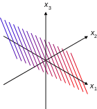
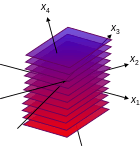
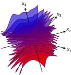
When the number of variables is two, a level set is generically a curve, called a level curve, contour line, or isoline. So a level curve is the set of all real-valued solutions of an equation in two variables x₁ and x₂. When n = 3, a level set is called a level surface (see also isosurface), and for higher values of n the level set is a level hypersurface. So a level surface is the set of all real-valued roots of an equation in three variables x₁, x₂ and x₃, and a level hypersurface is the set of all real-valued roots of an equation in n (n > 3) variables.

A level set is a special case of a fiber.

Alternative names

Intersections of a co-ordinate function's level surfaces with a trefoil knot. Red curves are closest to the viewer, while yellow curves are farthest.

Level sets show up in many applications, often under different names.

For example, an implicit curve is a level curve, which is considered independently of its neighbor curves, emphasizing that such a curve is defined by an implicit equation. Analogously, a level surface is sometimes called an implicit surface or an isosurface.

The name isocontour is also used, which means a contour of equal height. In various application areas, isocontours have received specific names, which indicate often the nature of the values of the considered function, such as isobar, isotherm, isogon, isochrone, isoquant and indifference curve.

Examples

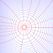
Consider the 2-dimensional Euclidean distance:

d(x,y)={\sqrt {x^{2}+y^{2}}}

A level set $L_{r}(d)$ of this function consists of those points that lie at a distance of $r$ from the origin, otherwise known as a circle. For example, $(3,4)\in L_{5}(d)$ , because $d(3,4)=5$ . Geometrically, this means that the point $(3,4)$ lies on the circle of radius 5 centered at the origin. More generally, a sphere in a metric space $(M,m)$ with radius $r$ centered at $x\in M$ can be defined as the level set $L_{r}(y\mapsto m(x,y))$ .

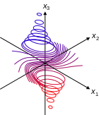
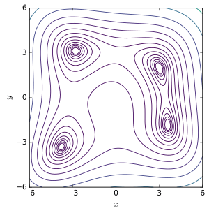
A second example is the plot of Himmelblau's function shown in the figure to the right. Each curve shown is a level curve of the function, and they are spaced logarithmically: if a curve represents $L_{x}$ , the curve directly "within" represents $L_{x/10}$ , and the curve directly "outside" represents $L_{10x}$ .

Log-spaced level curve plot of Himmelblau's function ^[1]

Level sets versus the gradient

Consider a function f whose graph looks like a hill. The blue curves are then the level sets. The red curves follow the direction of the gradient. In other words, the cautious hiker follows the blue paths, while the bold one the red paths.

Theorem. If the function

f

is differentiable, the gradient of

f

at a point is either zero, or perpendicular to the level set of

f

at that point.

To understand what this means, imagine that two hikers are at the same location on a mountain. One of them is bold, and he decides to go in the direction where the slope is steepest. The other one is more cautious; he does not want to either climb or descend, choosing a path which will keep him at the same height. In our analogy, the above theorem says that the two hikers will depart in directions perpendicular to one another.

A consequence of this theorem (and its proof) is that if $f$ is differentiable, a level set is a hypersurface and a manifold outside the critical points of $f$ . At a critical point, a level set may be reduced to a point (for example at a local extremum of $f$ ) or may have a singularity such as a self-intersection point or a cusp.

Sublevel and superlevel sets

A set of the form

L_{c}^{-}(f)=\left\{(x_{1},\cdots ,x_{n})\,\mid \,f(x_{1},\cdots ,x_{n})\leq c\right\}

is called a sublevel set of f (or, alternatively, a lower level set or trench of f).

L_{c}^{+}(f)=\left\{(x_{1},\cdots ,x_{n})\,\mid \,f(x_{1},\cdots ,x_{n})\geq c\right\}

is called a superlevel set of f.^[2]^[3] Sublevel sets are important in minimization theory. The boundness of some non-empty sublevel set and the lower-semicontinuity of the function implies that a function attains its minimum, by Weierstrass's theorem. The convexity of all the sublevel sets characterizes quasiconvex functions.^[4]

References

↑ Simionescu, P.A. (2011). "Some Advancements to Visualizing Constrained Functions and Inequalities of Two Variables". Transactions of the ASME - Journal of Computing and Information Science in Engineering. 11 (1). doi:10.1115/1.3570770.
↑ Voitsekhovskii, M.I. (2001) [1994], "L/l058220", in Hazewinkel, Michiel, Encyclopedia of Mathematics, Springer Science+Business Media B.V. / Kluwer Academic Publishers, ISBN 978-1-55608-010-4
↑ Weisstein, Eric W. "Level Set". MathWorld.
↑ Kiwiel, Krzysztof C. (2001). "Convergence and efficiency of subgradient methods for quasiconvex minimization". Mathematical Programming (Series A). 90 (1). Berlin, Heidelberg: Springer. pp. 1–25. doi:10.1007/PL00011414. ISSN 0025-5610. MR 1819784.

This article is issued from Wikipedia. The text is licensed under Creative Commons - Attribution - Sharealike. Additional terms may apply for the media files.

[1] Simionescu, P.A. (2011). "Some Advancements to Visualizing Constrained Functions and Inequalities of Two Variables". Transactions of the ASME - Journal of Computing and Information Science in Engineering. 11 (1). doi:10.1115/1.3570770.

[2] Voitsekhovskii, M.I. (2001) [1994], "L/l058220", in Hazewinkel, Michiel, Encyclopedia of Mathematics, Springer Science+Business Media B.V. / Kluwer Academic Publishers, ISBN 978-1-55608-010-4

[3] Weisstein, Eric W. "Level Set". MathWorld.

[4] Kiwiel, Krzysztof C. (2001). "Convergence and efficiency of subgradient methods for quasiconvex minimization". Mathematical Programming (Series A). 90 (1). Berlin, Heidelberg: Springer. pp. 1–25. doi:10.1007/PL00011414. ISSN 0025-5610. MR 1819784.