Lagrange multiplier

In mathematical optimization, the method of Lagrange multipliers (named after Joseph-Louis Lagrange^[1]) is a strategy for finding the local maxima and minima of a function subject to equality constraints (i.e., subject to the condition that one or more equations have to be satisfied exactly by the chosen values of the variables). The great advantage of this method is that it allows the optimization to be solved without explicit parameterization in terms of the constraints. As a result, the method of Lagrange multipliers is widely used to solve challenging constrained optimization problems.

The method can be summarized as follows:^[2]

isolate any possible singular point of the solution set of the constraining equations,
find all the stationary points of the Lagrange function,
establish which of those stationary points and singular points are global maxima (or minima, in case of minimization problems) of the objective function.

Single constraint

Figure 1: The red curve shows the constraint

g (x, y) = c

. The blue curves are contours of

f (x, y)

. The point where the red constraint tangentially touches a blue contour is the maximum of

f (x, y)

along the constraint, since

d 1 > d 2

.

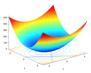
For the case of only one constraint and only two choice variables (as exemplified in Figure 1), consider the optimization problem

maximize

f (x, y)

subject to

g (x, y) = 0

.

(Sometimes an additive constant is shown separately rather than being included in g, in which case the constraint is written $g (x, y) = c$ , as in Figure 1.) We assume that both $f$ and $g$ have continuous first partial derivatives. We introduce a new variable ( $λ$ ) called a Lagrange multiplier and study the Lagrange function (or Lagrangian or Lagrangian expression) defined by

{\mathcal {L}}(x,y,\lambda )=f(x,y)-\lambda \cdot g(x,y),

where the $λ$ term may be either added or subtracted. If $f (x 0, y 0)$ is a maximum of $f (x, y)$ for the original constrained problem, then there exists $λ 0$ such that $(x 0, y 0, λ 0)$ is a stationary point for the Lagrange function (stationary points are those points where the partial derivatives of ${\mathcal {L}}$ are zero). However, not all stationary points yield a solution of the original problem. Thus, the method of Lagrange multipliers yields a necessary condition for optimality in constrained problems.^[3]^[4]^[5]^[6]^[7] Sufficient conditions for a minimum or maximum also exist, but if a particular candidate solution satisfies the sufficient conditions, it is only guaranteed that that solution is the best one locally – that is, it is better than any permissible nearby points. The global optimum can be found by comparing the values of the original objective function at the points satisfying the necessary and locally sufficient conditions.

The method of Lagrange multipliers relies on the intuition that at a maximum, $f (x, y)$ cannot be increasing in the direction of any neighboring point where $g = 0$ . If it were, we could walk along $g = 0$ to get higher, meaning that the starting point wasn't actually the maximum.

We can visualize contours of $f$ given by $f (x, y) = d$ for various values of $d$ , and the contour of $g$ given by $g (x, y) = 0$ .

Suppose we walk along the contour line with $g = 0$ . We are interested in finding points where $f$ does not change as we walk, since these points might be maxima. There are two ways this could happen: First, we could be following a contour line of $f$ , since by definition $f$ does not change as we walk along its contour lines. This would mean that the contour lines of $f$ and $g$ are parallel here. The second possibility is that we have reached a "level" part of $f$ , meaning that $f$ does not change in any direction.

To check the first possibility (we are following a contour line of $f$ ), notice that since the gradient of a function is perpendicular to the contour lines, the contour lines of $f$ and $g$ are parallel if and only if the gradients of $f$ and $g$ are parallel. Thus we want points $(x, y)$ where $g (x, y) = 0$ and

\nabla _{x,y}f=\lambda \nabla _{x,y}g,

for some $λ$

where

\nabla _{x,y}f=\left({\frac {\partial f}{\partial x}},{\frac {\partial f}{\partial y}}\right),\qquad \nabla _{x,y}g=\left({\frac {\partial g}{\partial x}},{\frac {\partial g}{\partial y}}\right).

are the respective gradients. The constant $λ$ is required because although the two gradient vectors are parallel, the magnitudes of the gradient vectors are generally not equal. This constant is called the Lagrange multiplier. (In some conventions $λ$ is preceded by a minus sign).

Notice that this method also solves the second possibility, that $f$ is level: if $f$ is level, then its gradient is zero, and setting $λ = 0$ is a solution regardless of $\nabla _{x,y}g$ .

To incorporate these conditions into one equation, we introduce an auxiliary function

{\mathcal {L}}(x,y,\lambda )=f(x,y)-\lambda \cdot g(x,y),

and solve

\nabla _{x,y,\lambda }{\mathcal {L}}(x,y,\lambda )=0.

Note that this amounts to solving three equations in three unknowns. This is the method of Lagrange multipliers. Note that $\nabla _{\lambda }{\mathcal {L}}(x,y,\lambda )=0$ implies $g (x, y) = 0$ . To summarize

\nabla _{x,y,\lambda }{\mathcal {L}}(x,y,\lambda )=0\iff {\begin{cases}\nabla _{x,y}f(x,y)=\lambda \nabla _{x,y}g(x,y)\\g(x,y)=0\end{cases}}

The method generalizes readily to functions on $n$ variables

\nabla _{x_{1},\dots ,x_{n},\lambda }{\mathcal {L}}(x_{1},\dots ,x_{n},\lambda )=0

which amounts to solving $n+1$ equations in $n+1$ unknowns.

The constrained extrema of $f$ are critical points of the Lagrangian ${\mathcal {L}}$ , but they are not necessarily local extrema of ${\mathcal {L}}$ (see Example 2 below).

One may reformulate the Lagrangian as a Hamiltonian, in which case the solutions are local minima for the Hamiltonian. This is done in optimal control theory, in the form of Pontryagin's minimum principle.

The fact that solutions of the Lagrangian are not necessarily extrema also poses difficulties for numerical optimization. This can be addressed by computing the magnitude of the gradient, as the zeros of the magnitude are necessarily local minima, as illustrated in the numerical optimization example.

Multiple constraints

Figure 2: A paraboloid constrained along two intersecting lines.

Figure 3: Contour map of Figure 2.

The method of Lagrange multipliers can be extended to solve problems with multiple constraints using a similar argument. Consider a paraboloid subject to two line constraints that intersect at a single point. As the only feasible solution, this point is obviously a constrained extremum. However, the level set of $f$ is clearly not parallel to either constraint at the intersection point (see Figure 3); instead, it is a linear combination of the two constraints' gradients. In the case of multiple constraints, that will be what we seek in general: the method of Lagrange seeks points not at which the gradient of $f$ is multiple of any single constraint's gradient necessarily, but in which it is a linear combination of all the constraints' gradients.

Concretely, suppose we have $M$ constraints and are walking along the set of points satisfying $g_{i}(\mathbf {x} )=0,i=1,\dots ,M$ . Every point $\mathbf {x}$ on the contour of a given constraint function $g_{i}$ has a space of allowable directions: the space of vectors perpendicular to $\nabla g_{i}(\mathbf {x} )$ . The set of directions that are allowed by all constraints is thus the space of directions perpendicular to all of the constraints' gradients. Denote this space of allowable moves by $A$ and denote the span of the constraints' gradients by $S$ . Then $A=S^{\perp }$ , the space of vectors perpendicular to every element of $S$ .

We are still interested in finding points where $f$ does not change as we walk, since these points might be (constrained) extrema. We therefore seek $\mathbf {x}$ such that any allowable direction of movement away from $\mathbf {x}$ is perpendicular to $\nabla f(\mathbf{x})$ (otherwise we could increase $f$ by moving along that allowable direction). In other words, $\nabla f(\mathbf {x} )\in A^{\perp }=S$ . Thus there are scalars $λ 1, λ 2, ..., λ M$ such that

\nabla f(\mathbf {x} )=\sum _{k=1}^{M}\lambda _{k}\nabla g_{k}(\mathbf {x} )\quad \iff \quad \nabla f(\mathbf {x} )-\sum _{k=1}^{M}{\lambda _{k}\nabla g_{k}(\mathbf {x} )}=0.

These scalars are the Lagrange multipliers. We now have $M$ of them, one for every constraint.

As before, we introduce an auxiliary function

{\mathcal {L}}\left(x_{1},\ldots ,x_{n},\lambda _{1},\ldots ,\lambda _{M}\right)=f\left(x_{1},\ldots ,x_{n}\right)-\sum \limits _{k=1}^{M}{\lambda _{k}g_{k}\left(x_{1},\ldots ,x_{n}\right)}

and solve

\nabla _{x_{1},\ldots ,x_{n},\lambda _{1},\ldots ,\lambda _{M}}{\mathcal {L}}(x_{1},\ldots ,x_{n},\lambda _{1},\ldots ,\lambda _{M})=0\iff {\begin{cases}\nabla f(\mathbf {x} )-\sum _{k=1}^{M}{\lambda _{k}\,\nabla g_{k}(\mathbf {x} )}=0\\g_{1}(\mathbf {x} )=\cdots =g_{M}(\mathbf {x} )=0\end{cases}}

which amounts to solving $n+M$ equations in $n+M$ unknowns.

The method of Lagrange multipliers is generalized by the Karush–Kuhn–Tucker conditions, which can also take into account inequality constraints of the form $h (x) \leq c$ .

Modern formulation via differentiable manifolds

The problem of finding the local maxima and minima subject to equality constraints can be generalized to finding local maxima and minima on a differentiable manifold. Let $M$ be a smooth manifold embedded in $\mathbb {R} ^{n}$ with codimension $p$ . Suppose $f\colon \mathbb {R} ^{n}\to \mathbb {R}$ is a differentiable function that we wish to maximize on $M$ . By an extension of Fermat's theorem the local maxima occur at points where the exterior derivative $df$ vanishes.^[8] In particular, supposing we have a local coordinate chart $\varphi \colon U\to \mathbb {R} ^{n-p}$ for $U\subseteq M$ , the extrema of $f$ are a subset of the critical points of the function $f_{\varphi }=f\circ \varphi ^{-1}\colon V\to \mathbb {R}$ , where $V$ is the image of $\varphi$ . However, it is often difficult to compute $\varphi ^{-1}$ explicitly. The entire method of Lagrange multipliers reduces to the idea of skipping that step and finding the zeros of $df_{\varphi }$ directly.

It remains to show that this notion of critical point is well defined. Suppose that $\varphi$ and $\psi$ are charts on $M$ whose domains both contain some point $y$ . The chain rule implies that $\varphi (y)$ is a critical point of $f_{\varphi }$ if and only if $\psi (y)$ is a critical point of $f_{\psi }$ . Indeed,

f_{\varphi }=f\circ \varphi ^{-1}=f\circ (\psi ^{-1}\circ \psi )\circ \varphi ^{-1}=f_{\psi }\circ (\psi \circ \varphi ^{-1}).

The composition $\psi \circ \varphi ^{-1}$ is a transition map for $M$ and therefore is a diffeomorphism. It follows that

D_{\varphi (y)}f_{\varphi }=D_{\psi (y)}f_{\psi }\circ D_{\varphi (y)}(\psi \circ \varphi ^{-1}),

so $D_{\varphi (y)}f_{\varphi }$ is the $0$ map if and only if the same is true of $D_{\psi (y)}f_{\psi }$ . Formally, we're looking for points $y\in M$ such that for some (and hence any) chart $\varphi$ containing $y$ , $\varphi (y)$ is a critical point of $f_{\varphi }$ .^[9]

Suppose the manifold $M$ is defined by a smooth level set function $g\colon \mathbb {R} ^{n}\to \mathbb {R} ^{p}$ as $M=\{x\in \mathbb {R} ^{n}:g(x)=c\}$ , with $c\in \mathbb {R} ^{p}$ and $g$ a submersion. It follows from the construction in the level set theorem that the image of $D_{x}\varphi ^{-1}$ is $\ker D_{\varphi ^{-1}(x)}g\subseteq \mathbb {R} ^{n}$ , where we tacitly identify $T_{\varphi ^{-1}(x)}M$ with a subspace of $\mathbb {R} ^{n}$ via the inclusion map on $M$ . Therefore,

0=D_{x}f_{\varphi }=D_{x}(f\circ \varphi ^{-1})=D_{\varphi ^{-1}(x)}f\circ D_{x}\varphi ^{-1}

if and only if

\ker D_{y}g\subseteq \ker D_{y}f

writing $y$ for $\varphi ^{-1}(x)$ . Again we can naturally interpret elements of $U$ , particularly $y$ itself, as points in $\mathbb {R} ^{n}$ via the inclusion map on $M$ .

By a combination of the first and third isomorphism theorems, the image of $D_{y}f$ must be isomorphic to a subspace of the image of $D_{y}g$ . It follows that there exists a linear map ${\mathcal {L}}\colon \mathbb {R} ^{p}\to \mathbb {R}$ such that ${\mathcal {L}}\circ D_{y}g=D_{y}f$ . As a linear map, ${\mathcal L}$ must satisfy ${\mathcal {L}}(x)=\lambda x$ for a fixed $\lambda \in \mathbb {R} ^{p}$ , so finding a critical point of $f_{\varphi }$ is equivalent to solving the system of equations

\lambda D_{y}g=D_{y}f

g(y)=c

in the variables $y\in {\mathbb {R}}^{{n}}$ and $\lambda \in \mathbb {R} ^{p}$ . This is in general a non-linear system of $n+p$ equations and $n+p$ unknowns.

Finding local maxima of a function $f:U\to \mathbb {R}$ is done by finding all points $x\in U$ such that $D_{x}f=0$ then checking whether all the eigenvalues of the Hessian $H_{x}f$ are negative. (Note that the maxima may not exist even if $f$ is continuous because $U$ is open, and also note that the conditions checked here are sufficient but not necessary for optimality.) Setting $D_{x}f=0$ is a non-linear problem and in general, arbitrarily difficult. After finding the critical points, checking the eigenvalues is a linear problem and thus easy.

Interpretation of the Lagrange multipliers

Often the Lagrange multipliers have an interpretation as some quantity of interest. For example, if the Lagrangian expression is

{\mathcal {L}}(x_{1},x_{2},\dots ;\lambda _{1},\lambda _{2},\dots )=f(x_{1},x_{2},\dots )+\lambda _{1}(c_{1}-g_{1}(x_{1},x_{2},\dots ))+\lambda _{2}(c_{2}-g_{2}(x_{1},x_{2},\dots ))+\cdots

then

{\frac {\partial {\mathcal {L}}}{\partial c_{k}}}=\lambda _{k}.

So, $λ k$ is the rate of change of the quantity being optimized as a function of the constraint parameter. As examples, in Lagrangian mechanics the equations of motion are derived by finding stationary points of the action, the time integral of the difference between kinetic and potential energy. Thus, the force on a particle due to a scalar potential, $F = -\nabla V$ , can be interpreted as a Lagrange multiplier determining the change in action (transfer of potential to kinetic energy) following a variation in the particle's constrained trajectory. In control theory this is formulated instead as costate equations.

Moreover, by the envelope theorem the optimal value of a Lagrange multiplier has an interpretation as the marginal effect of the corresponding constraint constant upon the optimal attainable value of the original objective function: if we denote values at the optimum with an asterisk, then it can be shown that

{\frac {{\text{d}}f(x_{1}^{*}(c_{1},c_{2},\dots ),x_{2}^{*}(c_{1},c_{2},\dots ),\dots )}{{\text{d}}c_{k}}}=\lambda _{k}^{*}.

For example, in economics the optimal profit to a player is calculated subject to a constrained space of actions, where a Lagrange multiplier is the change in the optimal value of the objective function (profit) due to the relaxation of a given constraint (e.g. through a change in income); in such a context $λ *$ is the marginal cost of the constraint, and is referred to as the shadow price.

Sufficient conditions

Sufficient conditions for a constrained local maximum or minimum can be stated in terms of a sequence of principal minors (determinants of upper-left-justified sub-matrices) of the bordered Hessian matrix of second derivatives of the Lagrangian expression.^[10]

Examples

Example 1

Illustration of the constrained optimization problem

Example 1a

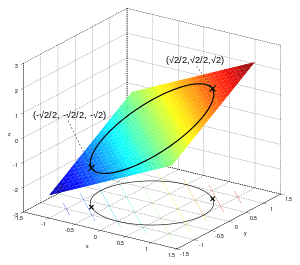
Suppose we wish to maximize $f(x,y)=x+y$ subject to the constraint $x^{2}+y^{2}=1$ . The feasible set is the unit circle, and the level sets of $f$ are diagonal lines (with slope −1), so we can see graphically that the maximum occurs at $\left({\tfrac {\sqrt {2}}{2}},{\tfrac {\sqrt {2}}{2}}\right)$ , and that the minimum occurs at $\left(-{\tfrac {\sqrt {2}}{2}},-{\tfrac {\sqrt {2}}{2}}\right)$ .

For the method of Lagrange multipliers, the constraint is

g(x,y)=x^{2}+y^{2}-1,

hence

{\begin{aligned}{\mathcal {L}}(x,y,\lambda )&=f(x,y)+\lambda \cdot g(x,y)\\&=x+y+\lambda (x^{2}+y^{2}-1).\end{aligned}}

Now we can calculate the gradient:

{\begin{aligned}\nabla _{x,y,\lambda }{\mathcal {L}}(x,y,\lambda )&=\left({\frac {\partial {\mathcal {L}}}{\partial x}},{\frac {\partial {\mathcal {L}}}{\partial y}},{\frac {\partial {\mathcal {L}}}{\partial \lambda }}\right)\\&=\left(1+2\lambda x,1+2\lambda y,x^{2}+y^{2}-1\right)\end{aligned}}

and therefore:

\nabla _{x,y,\lambda }{\mathcal {L}}(x,y,\lambda )=0\quad \Leftrightarrow \quad {\begin{cases}1+2\lambda x=0\\1+2\lambda y=0\\x^{2}+y^{2}-1=0\end{cases}}

Notice that the last equation is the original constraint.

The first two equations yield

x=y=-{\frac {1}{2\lambda }},\qquad \lambda \neq 0.

By substituting into the last equation we have:

{\frac {1}{4\lambda ^{2}}}+{\frac {1}{4\lambda ^{2}}}-1=0,

so

\lambda =\pm {\frac {1}{\sqrt {2}}},

which implies that the stationary points of ${\mathcal {L}}$ are

\left({\tfrac {\sqrt {2}}{2}},{\tfrac {\sqrt {2}}{2}},-{\tfrac {1}{\sqrt {2}}}\right),\qquad \left(-{\tfrac {\sqrt {2}}{2}},-{\tfrac {\sqrt {2}}{2}},{\tfrac {1}{\sqrt {2}}}\right).

Evaluating the objective function $f$ at these points yields

f\left({\tfrac {\sqrt {2}}{2}},{\tfrac {\sqrt {2}}{2}}\right)={\sqrt {2}},\qquad f\left(-{\tfrac {\sqrt {2}}{2}},-{\tfrac {\sqrt {2}}{2}}\right)=-{\sqrt {2}}.

Thus the constrained maximum is ${\sqrt {2}}$ and the constrained minimum is $-{\sqrt {2}}$ .

Example 1b

Now we modify the objective function of Example 1a so that we minimize $f(x,y)=(x+y)^2$ instead of $f(x,y)=x+y,$ again along the circle $g(x,y)=x^{2}+y^{2}-1=0$ . Now the level sets of f are still lines of slope −1, and the points on the circle tangent to these level sets are again $({\sqrt {2}}/2,{\sqrt {2}}/2)$ and $(-{\sqrt {2}}/2,-{\sqrt {2}}/2)$ . These tangency points are maxima of f.

On the other hand, the minima occur on the level set for f = 0 (since by its construction f cannot take negative values), at $(\sqrt{2}/2,-\sqrt{2}/2)$ and $(-{\sqrt {2}}/2,{\sqrt {2}}/2)$ , where the level curves of f are not tangent to the constraint. The condition that $\nabla f=\lambda\nabla g$ correctly identifies all four points as extrema; the minima are characterized in particular by $\lambda =0.$

Example 2

Illustration of the constrained optimization problem

In this example we will deal with some more strenuous calculations, but it is still a single constraint problem.

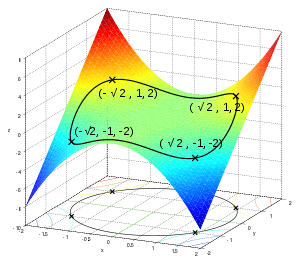
Suppose we want to find the maximum values of

f(x,y)=x^{2}y

with the condition that the $x$ and $y$ coordinates lie on the circle around the origin with radius √3, that is, subject to the constraint

g(x,y)=x^{2}+y^{2}-3=0.

As there is just a single constraint, we will use only one multiplier, say $λ$ .

The constraint $g (x, y)$ is identically zero on the circle of radius √3. See that any multiple of $g (x, y)$ may be added to $f (x, y)$ leaving $f (x, y)$ unchanged in the region of interest (on the circle where our original constraint is satisfied).

Apply the ordinary Langrange multiplier method. Let:

{\begin{aligned}{\mathcal {L}}(x,y,\lambda )&=f(x,y)+\lambda \cdot g(x,y)\\&=x^{2}y+\lambda (x^{2}+y^{2}-3)\end{aligned}}

Now we can calculate the gradient:

{\begin{aligned}\nabla _{x,y,\lambda }{\mathcal {L}}(x,y,\lambda )&=\left({\frac {\partial {\mathcal {L}}}{\partial x}},{\frac {\partial {\mathcal {L}}}{\partial y}},{\frac {\partial {\mathcal {L}}}{\partial \lambda }}\right)\\&=\left(2xy+2\lambda x,x^{2}+2\lambda y,x^{2}+y^{2}-3\right)\end{aligned}}

And therefore:

\nabla _{x,y,\lambda }{\mathcal {L}}(x,y,\lambda )=0\quad \Leftrightarrow \quad {\begin{cases}2xy+2\lambda x=0\\x^{2}+2\lambda y=0\\x^{2}+y^{2}-3=0\end{cases}}\quad \Leftrightarrow \quad {\begin{cases}x(y+\lambda )=0&(i)\\x^{2}=-2\lambda y&(ii)\\x^{2}+y^{2}=3&(iii)\end{cases}}

Notice that (iii) is just the original constraint. (i) implies $x = 0$ or $λ = - y$ . If $x = 0$ then $y=\pm {\sqrt {3}}$ by (iii) and consequently $λ = 0$ from (ii). If $λ = - y$ , substituting in (ii) we get $x 2 = 2 y 2$ . Substituting this in (iii) and solving for $y$ gives $y = \pm1$ . Thus there are six critical points of ${\mathcal {L}}$ :

({\sqrt {2}},1,-1);\quad (-{\sqrt {2}},1,-1);\quad ({\sqrt {2}},-1,1);\quad (-{\sqrt {2}},-1,1);\quad (0,{\sqrt {3}},0);\quad (0,-{\sqrt {3}},0).

Evaluating the objective at these points, we find that

f(\pm {\sqrt {2}},1)=2;\quad f(\pm {\sqrt {2}},-1)=-2;\quad f(0,\pm {\sqrt {3}})=0.

Therefore, the objective function attains the global maximum (subject to the constraints) at $(\pm {\sqrt {2}},1)$ and the global minimum at $(\pm {\sqrt {2}},-1).$ The point $(0,{\sqrt {3}})$ is a local minimum of f and $(0,-{\sqrt {3}})$ is a local maximum of f, as may be determined by consideration of the Hessian matrix of ${\mathcal {L}}(x,y,0)$ .

Note that while $({\sqrt {2}},1,-1)$ is a critical point of ${\mathcal {L}}$ , it is not a local extremum of ${\mathcal {L}}.$ We have

{\mathcal {L}}\left({\sqrt {2}}+\varepsilon ,1,-1+\delta \right)=2+\delta \left(\varepsilon ^{2}+\left(2{\sqrt {2}}\right)\varepsilon \right).

Given any neighborhood of $({\sqrt {2}},1,-1)$ , we can choose a small positive $\varepsilon$ and a small $\delta$ of either sign to get ${\mathcal {L}}$ values both greater and less than $2$ . This can also be seen from the fact that the Hessian matrix of ${\mathcal {L}}$ evaluated at this point (or indeed at any of the critical points) is an indefinite matrix. Each of the critical points of ${\mathcal {L}}$ is a saddle point of ${\mathcal {L}}.$

Example 3: Entropy

Suppose we wish to find the discrete probability distribution on the points $\{p_{1},p_{2},\ldots ,p_{n}\}$ with maximal information entropy. This is the same as saying that we wish to find the least structured probability distribution on the points $\{p_{1},p_{2},\cdots ,p_{n}\}$ . In other words, we wish to maximize the Shannon entropy equation:

f(p_{1},p_{2},\ldots ,p_{n})=-\sum _{j=1}^{n}p_{j}\log _{2}p_{j}.

For this to be a probability distribution the sum of the probabilities $p_{i}$ at each point $x_{i}$ must equal 1, so our constraint is:

g(p_{1},p_{2},\ldots ,p_{n})=\sum _{j=1}^{n}p_{j}=1.

We use Lagrange multipliers to find the point of maximum entropy, ${\vec {p}}^{\,*}$ , across all discrete probability distributions ${\vec {p}}$ on $\{x_{1},x_{2},\ldots ,x_{n}\}$ . We require that:

\left.{\frac {\partial }{\partial {\vec {p}}}}(f+\lambda (g-1))\right|_{{\vec {p}}={\vec {p}}^{\,*}}=0,

which gives a system of $n$ equations, $k=1,\ldots ,n$ , such that:

\left.{\frac {\partial }{\partial p_{k}}}\left\{-\left(\sum _{j=1}^{n}p_{j}\log _{2}p_{j}\right)+\lambda \left(\sum _{j=1}^{n}p_{j}-1\right)\right\}\right|_{p_{k}=p_{k}^{*}}=0.

Carrying out the differentiation of these $n$ equations, we get

-\left({\frac {1}{\ln 2}}+\log _{2}p_{k}^{*}\right)+\lambda =0.

This shows that all $p_{k}^{*}$ are equal (because they depend on $λ$ only). By using the constraint

\sum _{j}p_{j}=1,

we find

p_{k}^{*}={\frac {1}{n}}.

Hence, the uniform distribution is the distribution with the greatest entropy, among distributions on $n$ points.

Example 4: Numerical optimization

Lagrange multipliers cause the critical points to occur at saddle points.

The magnitude of the gradient can be used to force the critical points to occur at local minima.

The critical points of Lagrangians occur at saddle points, rather than at local maxima (or minima).^[11] Unfortunately, many numerical optimization techniques, such as hill climbing, gradient descent, some of the quasi-Newton methods, among others, are designed to find local maxima (or minima) and not saddle points. For this reason, one must either modify the formulation to ensure that it's a minimization problem (for example, by extremizing the square of the gradient of the Lagrangian as below), or else use an optimization technique that finds stationary points (such as Newton's method without an extremum seeking line search) and not necessarily extrema.

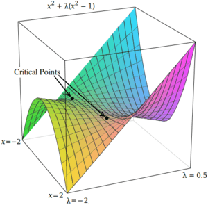
As a simple example, consider the problem of finding the value of $x$ that minimizes $f(x)=x^{2}$ , constrained such that $x^{2}=1$ . (This problem is somewhat pathological because there are only two values that satisfy this constraint, but it is useful for illustration purposes because the corresponding unconstrained function can be visualized in three dimensions.)

Using Lagrange multipliers, this problem can be converted into an unconstrained optimization problem:

{\mathcal {L}}(x,\lambda )=x^{2}+\lambda (x^{2}-1).

The two critical points occur at saddle points where $x = 1$ and $x = -1$ .

In order to solve this problem with a numerical optimization technique, we must first transform this problem such that the critical points occur at local minima. This is done by computing the magnitude of the gradient of the unconstrained optimization problem.

First, we compute the partial derivative of the unconstrained problem with respect to each variable:

{\frac {\partial {\mathcal {L}}}{\partial x}}=2x+2x\lambda

{\frac {\partial {\mathcal {L}}}{\partial \lambda }}=x^{2}-1.

If the target function is not easily differentiable, the differential with respect to each variable can be approximated as

{\frac {\partial {\mathcal {L}}}{\partial x}}\approx {\frac {{\mathcal {L}}(x+\varepsilon ,\lambda )-{\mathcal {L}}(x,\lambda )}{\varepsilon }},

{\frac {\partial {\mathcal {L}}}{\partial \lambda }}\approx {\frac {{\mathcal {L}}(x,\lambda +\varepsilon )-{\mathcal {L}}(x,\lambda )}{\varepsilon }},

where $\varepsilon$ is a small value.

Next, we compute the magnitude of the gradient, which is the square root of the sum of the squares of the partial derivatives:

h(x,\lambda )={\sqrt {(2x+2x\lambda )^{2}+(x^{2}-1)^{2}}}\approx {\sqrt {\left({\frac {{\mathcal {L}}(x+\varepsilon ,\lambda )-{\mathcal {L}}(x,\lambda )}{\varepsilon }}\right)^{2}+\left({\frac {{\mathcal {L}}(x,\lambda +\varepsilon )-{\mathcal {L}}(x,\lambda )}{\varepsilon }}\right)^{2}}}.

(Since magnitude is always non-negative, optimizing over the squared-magnitude is equivalent to optimizing over the magnitude. Thus, the ''square root" may be omitted from these equations with no expected difference in the results of optimization.)

The critical points of $h$ occur at $x = 1$ and $x = -1$ , just as in ${\mathcal {L}}$ . Unlike the critical points in ${\mathcal {L}}$ , however, the critical points in $h$ occur at local minima, so numerical optimization techniques can be used to find them.

Applications

Control theory

In optimal control theory, the Lagrange multipliers are interpreted as costate variables, and Lagrange multipliers are reformulated as the minimization of the Hamiltonian, in Pontryagin's minimum principle.

Nonlinear programming

The Lagrange multiplier method has several generalizations. In nonlinear programming there are several multiplier rules, e.g., the Carathéodory–John Multiplier Rule and the Convex Multiplier Rule, for inequality constraints.^[12]

References

↑ Mécanique Analytique sect. IV, 2 vols. Paris, 1811 https://archive.org/details/mcaniqueanalyt01lagr
↑ Bramanti, Marco (2004). Matematica: Calcolo Infinitesimale e Algebra Lineare (2nd ed.). Bologna: Zanichelli. pp. 462–468. ISBN 978-88-08-07547-5.
↑ Bertsekas 1999
↑ Vapnyarskii, I.B. (2001) [1994], "Lagrange multipliers", in Hazewinkel, Michiel, Encyclopedia of Mathematics, Springer Science+Business Media B.V. / Kluwer Academic Publishers, ISBN 978-1-55608-010-4 .
↑ Lasdon 1970, pp. xi+523
↑ Hiriart-Urruty & Lemaréchal 1993, pp. 136–193 (and Bibliographical comments on pp. 334–335)
↑ Lemaréchal, Claude (2001). "Lagrangian relaxation". In Jünger, Michael; Naddef, Denis. Computational combinatorial optimization: Papers from the Spring School held in Schloß Dagstuhl, May 15–19, 2000. Lecture Notes in Computer Science. 2241. Berlin: Springer-Verlag. pp. 112–156. doi:10.1007/3-540-45586-8_4. ISBN 3-540-42877-1. MR 1900016.
↑ Lafontaine, p. 70
↑ Lee, Jeffrey M. (2009). Manifolds and Differential Geometry. Providence: American Mathematical Society. p. 23. ISBN 978-0-8218-4815-9. Lee discusses a property being true specifically for some "and hence any" chart on a manifold.
↑ Chiang 1984, p. 386
↑ Heath 2005, p. 203
↑ Pourciau, Bruce H. (1980). "Modern Multiplier Rules". The American Mathematical Monthly. 87 (6): 433–452. doi:10.2307/2320250. JSTOR 2320250.

Sources

Bertsekas, Dimitri P. (1999). Nonlinear Programming (Second ed.). Cambridge, MA.: Athena Scientific. ISBN 1-886529-00-0.
Chiang, Alpha C. (1984). Fundamental Methods of Mathematical Economics (third ed.). McGraw-Hill. ISBN 9757860069.
Heath, Michael T. (2005). Scientific Computing: An Introductory Survey. McGraw-Hill. p. 203. ISBN 978-0-07-124489-3.
Hiriart-Urruty, Jean-Baptiste; Lemaréchal, Claude (1993). "XII Abstract duality for practitioners". Convex analysis and minimization algorithms, Volume II: Advanced theory and bundle methods. Grundlehren der Mathematischen Wissenschaften [Fundamental Principles of Mathematical Sciences]. 306. Berlin: Springer-Verlag. ISBN 3-540-56852-2. MR 1295240.
Lafontaine, Jacques. An Introduction to Differential Manifolds. Springer. p. 70. ISBN 9783319207353.
Lasdon, Leon S. (1970). Optimization theory for large systems. Macmillan series in operations research. New York: The Macmillan Company. MR 0337317.
- Lasdon, Leon S. (2002). Optimization theory for large systems (reprint of the 1970 Macmillan ed.). Mineola, New York: Dover Publications, Inc. MR 1888251.

External links

Exposition

Conceptual introduction (plus a brief discussion of Lagrange multipliers in the calculus of variations as used in physics)
Lagrange Multipliers for Quadratic Forms With Linear Constraints by Kenneth H. Carpenter

For additional text and interactive applets

Simple explanation with an example of governments using taxes as Lagrange multipliers
Lagrange Multipliers without Permanent Scarring Explanation with focus on the intuition by Dan Klein
Geometric Representation of Method of Lagrange Multipliers Provides compelling insight in 2 dimensions that at a minimizing point, the direction of steepest descent must be perpendicular to the tangent of the constraint curve at that point. [Needs InternetExplorer/Firefox/Safari] Mathematica demonstration by Shashi Sathyanarayana
Applet
Video Lecture of Lagrange Multipliers
MIT OpenCourseware Video Lecture on Lagrange Multipliers from Multivariable Calculus course
Slides accompanying Bertsekas's nonlinear optimization text, with details on Lagrange multipliers (lectures 11 and 12)
Geometric idea behind Lagrange multipliers

This article is issued from Wikipedia. The text is licensed under Creative Commons - Attribution - Sharealike. Additional terms may apply for the media files.

[1] Mécanique Analytique sect. IV, 2 vols. Paris, 1811 https://archive.org/details/mcaniqueanalyt01lagr

[2] Bramanti, Marco (2004). Matematica: Calcolo Infinitesimale e Algebra Lineare (2nd ed.). Bologna: Zanichelli. pp. 462–468. ISBN 978-88-08-07547-5.

[3] Bertsekas 1999

[4] Vapnyarskii, I.B. (2001) [1994], "Lagrange multipliers", in Hazewinkel, Michiel, Encyclopedia of Mathematics, Springer Science+Business Media B.V. / Kluwer Academic Publishers, ISBN 978-1-55608-010-4 .

[5] Lasdon 1970, pp. xi+523

[6] Hiriart-Urruty & Lemaréchal 1993, pp. 136–193 (and Bibliographical comments on pp. 334–335)

[7] Lemaréchal, Claude (2001). "Lagrangian relaxation". In Jünger, Michael; Naddef, Denis. Computational combinatorial optimization: Papers from the Spring School held in Schloß Dagstuhl, May 15–19, 2000. Lecture Notes in Computer Science. 2241. Berlin: Springer-Verlag. pp. 112–156. doi:10.1007/3-540-45586-8_4. ISBN 3-540-42877-1. MR 1900016.

[8] Lafontaine, p. 70

[9] Lee, Jeffrey M. (2009). Manifolds and Differential Geometry. Providence: American Mathematical Society. p. 23. ISBN 978-0-8218-4815-9. Lee discusses a property being true specifically for some "and hence any" chart on a manifold.

[10] Chiang 1984, p. 386

[Heath2005-11] Heath 2005, p. 203

[12] Pourciau, Bruce H. (1980). "Modern Multiplier Rules". The American Mathematical Monthly. 87 (6): 433–452. doi:10.2307/2320250. JSTOR 2320250.