Karush–Kuhn–Tucker conditions

In mathematical optimization, the Karush–Kuhn–Tucker (KKT) conditions, also known as the Kuhn–Tucker conditions, are first-order necessary conditions for a solution in nonlinear programming to be optimal, provided that some regularity conditions are satisfied. Allowing inequality constraints, the KKT approach to nonlinear programming generalizes the method of Lagrange multipliers, which allows only equality constraints. The system of equations and inequalities corresponding to the KKT conditions is usually not solved directly, except in the few special cases where a closed-form solution can be derived analytically. In general, many optimization algorithms can be interpreted as methods for numerically solving the KKT system of equations and inequalities.^[1]

The KKT conditions were originally named after Harold W. Kuhn, and Albert W. Tucker, who first published the conditions in 1951.^[2] Later scholars discovered that the necessary conditions for this problem had been stated by William Karush in his master's thesis in 1939.^[3]^[4]

Nonlinear optimization problem

Consider the following nonlinear minimization or maximization problem:

Optimize

f(x)

subject to

g_{i}(x)\leq 0,

h_{j}(x)=0,

where $x$ is the optimization variable, $f$ is the objective or utility function, $g_{i}\ (i=1,\ldots ,m)$ are the inequality constraint functions, and $h_{j}\ (j=1,\ldots ,\ell )$ are the equality constraint functions. The numbers of inequality and equality constraints are denoted m and ℓ, respectively.

Necessary conditions

Suppose that the objective function $f:\mathbb {R} ^{n}\rightarrow \mathbb {R}$ and the constraint functions $g_{i}:\,\!\mathbb {R} ^{n}\rightarrow \mathbb {R}$ and $h_{j}:\,\!\mathbb {R} ^{n}\rightarrow \mathbb {R}$ are continuously differentiable at a point $x^{*}$ . If $x^{*}$ is a local optimum and the optimization problem satisfies some regularity conditions (see below), then there exist constants $\mu _{i}\ (i=1,\ldots ,m)$ and $\lambda _{j}\ (j=1,\ldots ,\ell )$ , called KKT multipliers, such that

Inequality constraint diagram for optimization problems

Stationarity: For maximizing f(x): $\nabla f(x^{*})=\sum _{i=1}^{m}\mu _{i}\nabla g_{i}(x^{*})+\sum _{j=1}^{\ell }\lambda _{j}\nabla h_{j}(x^{*}),$; For minimizing f(x): $-\nabla f(x^{*})=\sum _{i=1}^{m}\mu _{i}\nabla g_{i}(x^{*})+\sum _{j=1}^{\ell }\lambda _{j}\nabla h_{j}(x^{*}),$

Primal feasibility: $g_{i}(x^{*})\leq 0,{\text{ for }}i=1,\ldots ,m$; $h_{j}(x^{*})=0,{\text{ for }}j=1,\ldots ,\ell \,\!$

Dual feasibility: $\mu _{i}\geq 0,{\text{ for }}i=1,\ldots ,m$

Complementary slackness: $\mu _{i}g_{i}(x^{*})=0,{\text{ for }}\;i=1,\ldots ,m.$

In the particular case $m=0$ , i.e., when there are no inequality constraints, the KKT conditions turn into the Lagrange conditions, and the KKT multipliers are called Lagrange multipliers.

If some of the functions are non-differentiable, subdifferential versions of Karush–Kuhn–Tucker (KKT) conditions are available.^[5]

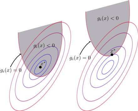
Regularity conditions (or constraint qualifications)

In order for a minimum point $x^{*}$ to satisfy the above KKT conditions, the problem should satisfy some regularity conditions; some common examples are tabulated here:

Constraint	Acronym	Statement
Linearity constraint qualification	LCQ	If $g_{i}$ and $h_{j}$ are affine functions, then no other condition is needed.
Linear independence constraint qualification	LICQ	The gradients of the active inequality constraints and the gradients of the equality constraints are linearly independent at $x^{*}$ .
Mangasarian-Fromovitz constraint qualification	MFCQ	The gradients of the equality constraints are linearly independent at $x^{}$ and there exists a vector $d\in \mathbb {R} ^{n}$ such that $\nabla g_{i}(x^{})^{\top }d<0$ for all active inequality constraints and $\nabla h_{j}(x^{*})^{\top }d=0$ for all equality constraints.^[6]
Constant rank constraint qualification	CRCQ	For each subset of the gradients of the active inequality constraints and the gradients of the equality constraints the rank at a vicinity of $x^{*}$ is constant.
Constant positive linear dependence constraint qualification	CPLD	For each subset of gradients of active inequality constraints and gradients of equality constraints, if the subset of vectors is linearly dependent at $x^{}$ with non-negative scalars associated with the inequality constraints, then it remain linearly dependent in a neighborhood of $x^{}$ .
Quasi-normality constraint qualification	QNCQ	If the gradients of the active inequality constraints and the gradients of the equality constraints are linearly dependent at $x^{}$ with associated multipliers $\lambda _{j}$ for equalities and $\mu _{i}\geq 0$ for inequalities, then there is no sequence $x_{k}\to x^{}$ such that $\lambda _{j}\neq 0\Rightarrow \lambda _{j}h_{j}(x_{k})>0$ and $\mu _{i}\neq 0\Rightarrow \mu _{i}g_{i}(x_{k})>0$ .
Slater condition	SC	For a convex problem (i.e., assuming minimization, $f,g_{i}$ are convex and $h_{j}$ is affine), there exists a point $x$ such that $h(x)=0$ and $g_{i}(x)<0$ .

It can be shown that

LICQ ⇒ MFCQ ⇒ CPLD ⇒ QNCQ

and

LICQ ⇒ CRCQ ⇒ CPLD ⇒ QNCQ

(and the converses are not true), although MFCQ is not equivalent to CRCQ.^[7] In practice weaker constraint qualifications are preferred since they provide stronger optimality conditions.

Sufficient conditions

In some cases, the necessary conditions are also sufficient for optimality. In general, the necessary conditions are not sufficient for optimality and additional information is necessary, such as the Second Order Sufficient Conditions (SOSC). For smooth functions, SOSC involve the second derivatives, which explains its name.

The necessary conditions are sufficient for optimality if the objective function $f$ of a maximization problem is a concave function, the inequality constraints $g_{j}$ are continuously differentiable convex functions and the equality constraints $h_{i}$ are affine functions.

It was shown by Martin in 1985 that the broader class of functions in which KKT conditions guarantees global optimality are the so-called Type 1 invex functions.^[8]^[9]

Second-order sufficient conditions

For smooth, non-linear optimization problems, a second order sufficient condition is given as follows. Consider $x^{*},\lambda ^{*},\mu ^{*}$ that find a local minimum using the Karush–Kuhn–Tucker conditions above. With $\mu ^{*}$ such that strict complementarity is held at $x^{*}$ (i.e. all $\mu _{i}>0$ ), then for all $s\neq 0$ such that

\left[{\frac {\partial g(x^{*})}{\partial x}},{\frac {\partial h(x^{*})}{\partial x}}\right]^{T}s=0

(where the bracketed expression is a row vector), the following equation must hold;

s'\nabla _{xx}^{2}L(x^{*},\lambda ^{*},\mu ^{*})s\geq 0

If the above condition is strictly met, the function is a strict constrained local minimum.

Economics

Often in mathematical economics the KKT approach is used in theoretical models in order to obtain qualitative results. For example,^[10] consider a firm that maximizes its sales revenue subject to a minimum profit constraint. Letting Q be the quantity of output produced (to be chosen), R(Q) be sales revenue with a positive first derivative and with a zero value at zero output, C(Q) be production costs with a positive first derivative and with a non-negative value at zero output, and $G_{\min }$ be the positive minimal acceptable level of profit, then the problem is a meaningful one if the revenue function levels off so it eventually is less steep than the cost function. The problem expressed in the previously given minimization form is

Minimize

-R(Q)

subject to

G_{\min }\leq R(Q)-C(Q)

Q\geq 0,

and the KKT conditions are

{\begin{aligned}&\left({\frac {{\text{d}}R}{{\text{d}}Q}}\right)(1+\mu )-\mu \left({\frac {{\text{d}}C}{{\text{d}}Q}}\right)\leq 0,\\[5pt]&Q\geq 0,\\[5pt]&Q\left[\left({\frac {{\text{d}}R}{{\text{d}}Q}}\right)(1+\mu )-\mu \left({\frac {{\text{d}}C}{{\text{d}}Q}}\right)\right]=0,\\[5pt]&R(Q)-C(Q)-G_{\min }\geq 0,\\[5pt]&\mu \geq 0,\\[5pt]&\mu [R(Q)-C(Q)-G_{\min }]=0.\end{aligned}}

Since Q = 0 would violate the minimum profit constraint, we have Q > 0 and hence the third condition implies that the first condition holds with equality. Solving that equality gives

{\frac {{\text{d}}R}{{\text{d}}Q}}={\frac {\mu }{1+\mu }}\left({\frac {{\text{d}}C}{{\text{d}}Q}}\right).

Because it was given that ${\text{d}}R/{\text{d}}Q$ and ${\text{d}}C/{\text{d}}Q$ are strictly positive, this inequality along with the non-negativity condition on $\mu$ guarantees that $\mu$ is positive and so the revenue-maximizing firm operates at a level of output at which marginal revenue ${\text{d}}R/{\text{d}}Q$ is less than marginal cost ${\text{d}}C/{\text{d}}Q$ — a result that is of interest because it contrasts with the behavior of a profit maximizing firm, which operates at a level at which they are equal.

Value function

If we reconsider the optimization problem as a maximization problem with constant inequality constraints,v.

{\text{Maximize }}\;f(x)

{\text{subject to }}\

g_{i}(x)\leq a_{i},h_{j}(x)=0.

The value function is defined as

V(a_{1},\ldots ,a_{n})=\sup \limits _{x}f(x)

{\text{subject to }}\

g_{i}(x)\leq a_{i},h_{j}(x)=0

j\in \{1,\ldots ,\ell \},i\in \{1,\ldots ,m\}.

(So the domain of V is $\{a\in \mathbb {R} ^{m}\mid {\text{for some }}x\in X,g_{i}(x)\leq a_{i},i\in \{1,\ldots ,m\}\}.$ )

Given this definition, each coefficient, $\mu _{i}$ , is the rate at which the value function increases as $a_{i}$ increases. Thus if each $a_{i}$ is interpreted as a resource constraint, the coefficients tell you how much increasing a resource will increase the optimum value of our function f. This interpretation is especially important in economics and is used, for instance, in utility maximization problems.

Generalizations

With an extra multiplier $\mu _{0}\geq 0$ , which may be zero (as long as $(\mu _{0},\mu ,\lambda )\neq 0$ ), in front of $\nabla f(x^{*})$ the KKT stationarity conditions turn into

{\begin{aligned}&\mu _{0}\,\nabla f(x^{*})+\sum _{i=1}^{m}\mu _{i}\,\nabla g_{i}(x^{*})+\sum _{j=1}^{\ell }\lambda _{j}\,\nabla h_{j}(x^{*})=0,\\[4pt]&\mu _{j}g_{i}(x^{*})=0,\quad i=1,\dots ,m,\end{aligned}}

which are called the Fritz John conditions. This optimality conditions holds without constraint qualifications and it is equivalent to the optimality condition KKT or (not-MFCQ).

The KKT conditions belong to a wider class of the first-order necessary conditions (FONC), which allow for non-smooth functions using subderivatives.

References

↑ Boyd, Stephen; Vandenberghe, Lieven (2004). Convex Optimization. Cambridge: Cambridge University Press. p. 244. ISBN 0-521-83378-7. MR 2061575.
↑ Kuhn, H. W.; Tucker, A. W. (1951). "Nonlinear programming". Proceedings of 2nd Berkeley Symposium. Berkeley: University of California Press. pp. 481–492. MR 0047303.
↑ W. Karush (1939). "Minima of Functions of Several Variables with Inequalities as Side Constraints". M.Sc. Dissertation. Dept. of Mathematics, Univ. of Chicago, Chicago, Illinois.
↑ Kjeldsen, Tinne Hoff (2000). "A contextualized historical analysis of the Kuhn-Tucker theorem in nonlinear programming: the impact of World War II". Historia Math. 27 (4): 331–361. doi:10.1006/hmat.2000.2289. MR 1800317.
↑ Ruszczyński, Andrzej (2006). Nonlinear Optimization. Princeton, NJ: Princeton University Press. ISBN 978-0691119151. MR 2199043.
↑ Dimitri Bertsekas (1999). Nonlinear Programming (2 ed.). Athena Scientific. pp. 329–330. ISBN 9781886529007.
↑ Rodrigo Eustaquio; Elizabeth Karas; Ademir Ribeiro. Constraint Qualification for Nonlinear Programming (PDF) (Technical report). Federal University of Parana.
↑ Martin, D. H. (1985). "The Essence of Invexity". J. Optim. Theory Appl. 47 (1): 65–76. doi:10.1007/BF00941316.
↑ Hanson, M. A. (1999). "Invexity and the Kuhn-Tucker Theorem". J. Math. Anal. Appl. 236 (2): 594–604. doi:10.1006/jmaa.1999.6484.
↑ Chiang, Alpha C. Fundamental Methods of Mathematical Economics, 3rd edition, 1984, pp. 750–752.

External links

This article is issued from Wikipedia. The text is licensed under Creative Commons - Attribution - Sharealike. Additional terms may apply for the media files.

[1] Boyd, Stephen; Vandenberghe, Lieven (2004). Convex Optimization. Cambridge: Cambridge University Press. p. 244. ISBN 0-521-83378-7. MR 2061575.

[2] Kuhn, H. W.; Tucker, A. W. (1951). "Nonlinear programming". Proceedings of 2nd Berkeley Symposium. Berkeley: University of California Press. pp. 481–492. MR 0047303.

[3] W. Karush (1939). "Minima of Functions of Several Variables with Inequalities as Side Constraints". M.Sc. Dissertation. Dept. of Mathematics, Univ. of Chicago, Chicago, Illinois.

[4] Kjeldsen, Tinne Hoff (2000). "A contextualized historical analysis of the Kuhn-Tucker theorem in nonlinear programming: the impact of World War II". Historia Math. 27 (4): 331–361. doi:10.1006/hmat.2000.2289. MR 1800317.

[5] Ruszczyński, Andrzej (2006). Nonlinear Optimization. Princeton, NJ: Princeton University Press. ISBN 978-0691119151. MR 2199043.

[6] Dimitri Bertsekas (1999). Nonlinear Programming (2 ed.). Athena Scientific. pp. 329–330. ISBN 9781886529007.

[7] Rodrigo Eustaquio; Elizabeth Karas; Ademir Ribeiro. Constraint Qualification for Nonlinear Programming (PDF) (Technical report). Federal University of Parana.

[8] Martin, D. H. (1985). "The Essence of Invexity". J. Optim. Theory Appl. 47 (1): 65–76. doi:10.1007/BF00941316.

[9] Hanson, M. A. (1999). "Invexity and the Kuhn-Tucker Theorem". J. Math. Anal. Appl. 236 (2): 594–604. doi:10.1006/jmaa.1999.6484.

[10] Chiang, Alpha C. Fundamental Methods of Mathematical Economics, 3rd edition, 1984, pp. 750–752.