Integration by parts

In calculus, and more generally in mathematical analysis, integration by parts or partial integration is a process that finds the integral of a product of functions in terms of the integral of their derivative and antiderivative. It is frequently used to transform the antiderivative of a product of functions into an antiderivative for which a solution can be more easily found. The rule can be derived in one line simply by integrating the product rule of differentiation.

If $u$ = $u (x)$ and $du$ = $u'(x) dx$ , while $v$ = $v (x)$ and $dv$ = $v'(x) dx$ , then integration by parts states that:

{\begin{aligned}\int _{a}^{b}u(x)v'(x)\,dx&=[u(x)v(x)]_{a}^{b}-\int _{a}^{b}u'(x)v(x)dx\\&=u(b)v(b)-u(a)v(a)-\int _{a}^{b}u'(x)v(x)\,dx\end{aligned}}

or more compactly:

\int u\,dv=uv-\int v\,du.\!

Mathematician Brook Taylor discovered integration by parts, first publishing the idea in 1715.^[1]^[2] More general formulations of integration by parts exist for the Riemann–Stieltjes and Lebesgue–Stieltjes integrals. The discrete analogue for sequences is called summation by parts.

Theorem

Product of two functions

The theorem can be derived as follows. Suppose u(x) and v(x) are two continuously differentiable functions. The product rule states (in Leibniz's notation):

{\frac {d}{dx}}{\Big (}u(x)v(x){\Big )}=v(x){\frac {d}{dx}}\left(u(x)\right)+u(x){\frac {d}{dx}}\left(v(x)\right).\!

Integrating both sides with respect to x,

\int {\frac {d}{dx}}\left(u(x)v(x)\right)\,dx=\int u'(x)v(x)\,dx+\int u(x)v'(x)\,dx

then applying the definition of indefinite integral,

u(x)v(x)=\int u'(x)v(x)\,dx+\int u(x)v'(x)\,dx

\int u(x)v'(x)\,dx=u(x)v(x)-\int u'(x)v(x)\,dx

gives the formula for integration by parts.

Since du and dv are differentials of a function of one variable x,

du=u'(x)dx\quad dv=v'(x)dx

\int u(x)\,dv=u(x)v(x)-\int v(x)\,du

The original integral ∫uv′ dx contains v′ (derivative of v); in order to apply the theorem, v (antiderivative of v′) must be found, and then the resulting integral ∫vu′ dx must be evaluated.

Extension to other cases

It is not actually necessary for u and v to be continuously differentiable. Integration by parts works if u is absolutely continuous and the function designated $v'$ is Lebesgue integrable (but not necessarily continuous).^[3] (If v' has a point of discontinuity then its antiderivative v may not have a derivative at that point.)

If the interval of integration is not compact, then it is not necessary for u to be absolutely continuous in the whole interval or for v ' to be Lebesgue integrable in the interval, as a couple of examples (in which u and v are continuous and continuously differentiable) will show. For instance, if

u(x)=\exp(x)/x^{2},\,v'(x)=\exp(-x)

u is not absolutely continuous on the interval $[1, +\infty)$ , but nevertheless

\int _{1}^{\infty }u(x)v'(x)\,dx=\left[u(x)v(x)\right]_{1}^{\infty }-\int _{1}^{\infty }u'(x)v(x)\,dx

so long as $\left[u(x)v(x)\right]_{1}^{\infty }$ is taken to mean the limit of $u(L)v(L)-u(1)v(1)$ as $L\to \infty$ and so long as the two terms on the right-hand side are finite. This is only true if we choose $v(x)=-\exp(-x).$ Similarly, if

u(x)=\exp(-x),\,v'(x)=x^{-1}\sin(x)

v' is not Lebesgue integrable on the interval $[1, +\infty)$ , but nevertheless

\int _{1}^{\infty }u(x)v'(x)\,dx=\left[u(x)v(x)\right]_{1}^{\infty }-\int _{1}^{\infty }u'(x)v(x)\,dx

with the same interpretation.

One can also easily come up with similar examples in which u and v are not continuously differentiable.

Further, if $f(x)$ is a function of bounded variation on the segment $[a,b],$ and $\varphi (x)$ is differentiable on $[a,b],$ then

$\int \limits _{a}^{b}f(x)\varphi '(x)\,dx=-\int \limits _{-\infty }^{+\infty }{\widetilde {\varphi }}(x)\,d({\widetilde {\chi }}_{[a,b]}(x){\widetilde {f}}(x)),$

where by $d(\chi _{[a,b]}(x){\widetilde {f}}(x))$ I denoted the signed measure corresponding to the function of bounded variation $\chi _{[a,b]}(x)f(x)$ , and functions ${\widetilde {f}},{\widetilde {\varphi }}$ are extensions of $f,\varphi$ to $\mathbb {R} ,$ which are respectively of bounded variation and differentiable.

Product of many functions

Integrating the product rule for three multiplied functions, u(x), v(x), w(x), gives a similar result:

\int _{a}^{b}uv\,dw=[uvw]_{a}^{b}-\int _{a}^{b}uw\,dv-\int _{a}^{b}vw\,du.

In general, for n factors

{\frac {d}{dx}}\left(\prod _{i=1}^{n}u_{i}(x)\right)=\sum _{j=1}^{n}\prod _{i\neq j}^{n}u_{i}(x){\frac {du_{j}(x)}{dx}},

which leads to

{\Bigl [}\prod _{i=1}^{n}u_{i}(x){\Bigr ]}_{a}^{b}=\sum _{j=1}^{n}\int _{a}^{b}\prod _{i\neq j}^{n}u_{i}(x)\,du_{j}(x),

where the product is of all functions except for the one differentiated in the same term.

Visualization

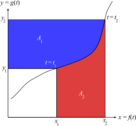
Graphical interpretation of the theorem. The pictured curve is parametrized by the variable t.

Consider a parametric curve by (x, y) = (f(t), g(t)). Assuming that the curve is locally one-to-one and integrable, we can define

x(y)=f(g^{-1}(y))

y(x)=g(f^{-1}(x))

The area of the blue region is

A_{1}=\int _{y_{1}}^{y_{2}}x(y)dy

Similarly, the area of the red region is

A_{2}=\int _{x_{1}}^{x_{2}}y(x)dx

The total area A₁ + A₂ is equal to the area of the bigger rectangle, x₂y₂, minus the area of the smaller one, x₁y₁:

\overbrace {\int _{y_{1}}^{y_{2}}x(y)dy} ^{A_{1}}+\overbrace {\int _{x_{1}}^{x_{2}}y(x)dx} ^{A_{2}}={\biggl .}x\cdot y(x){\biggl |}_{x_{1}}^{x_{2}}={\biggl .}y\cdot x(y){\biggl |}_{y_{1}}^{y_{2}}.

Or, in terms of t,

\int _{t_{1}}^{t_{2}}x(t)dy(t)+\int _{t_{1}}^{t_{2}}y(t)dx(t)={\biggl .}x(t)y(t){\biggl |}_{t_{1}}^{t_{2}}

Or, in terms of indefinite integrals, this can be written as

\int xdy+\int ydx=xy

Rearranging:

\int xdy=xy-\int ydx

Thus integration by parts may be thought of as deriving the area of the blue region from the area of rectangles and that of the red region.

This visualization also explains why integration by parts may help find the integral of an inverse function f⁻¹(x) when the integral of the function f(x) is known. Indeed, the functions x(y) and y(x) are inverses, and the integral ∫x dy may be calculated as above from knowing the integral ∫y dx. In particular, this explains use of integration by parts to integrate logarithm and inverse trigonometric functions.

Application to find antiderivatives

Strategy

Integration by parts is a heuristic rather than a purely mechanical process for solving integrals; given a single function to integrate, the typical strategy is to carefully separate this single function into a product of two functions u(x)v(x) such that the residual integral from the integration by parts formula is easier to evaluate than the single function. The following form is useful in illustrating the best strategy to take:

\int uv\ dx=u\int v\ dx-\int \left(u'\int v\ dx\right)\ dx.

Note that on the right-hand side, u is differentiated and v is integrated; consequently it is useful to choose u as a function that simplifies when differentiated, or to choose v as a function that simplifies when integrated. As a simple example, consider:

\int {\frac {\ln(x)}{x^{2}}}\ dx\ .

Since the derivative of ln(x) is 1/x, one makes (ln(x)) part u; since the antiderivative of 1/x² is -1/x, one makes 1/x²dx part dv. The formula now yields:

\int {\frac {\ln(x)}{x^{2}}}\ dx=-{\frac {\ln(x)}{x}}-\int {\biggl (}{\frac {1}{x}}{\biggr )}{\biggl (}-{\frac {1}{x}}{\biggr )}\ dx\ .

The antiderivative of −1/x² can be found with the power rule and is 1/x.

Alternatively, one may choose u and v such that the product u' (∫v dx) simplifies due to cancellation. For example, suppose one wishes to integrate:

\int \sec ^{2}(x)\cdot \ln {\Big (}{\bigl |}\sin(x){\bigr |}{\Big )}\ dx.

If we choose u(x) = ln(|sin(x)|) and v(x) = sec²x, then u differentiates to 1/ tan x using the chain rule and v integrates to tan x; so the formula gives:

\int \sec ^{2}(x)\cdot \ln {\Big (}{\bigl |}\sin(x){\bigr |}{\Big )}\ dx=\tan(x)\cdot \ln {\Big (}{\bigl |}\sin(x){\bigr |}{\Big )}-\int \tan(x)\cdot {\frac {1}{\tan(x)}}dx\ .

The integrand simplifies to 1, so the antiderivative is x. Finding a simplifying combination frequently involves experimentation.

In some applications, it may not be necessary to ensure that the integral produced by integration by parts has a simple form; for example, in numerical analysis, it may suffice that it has small magnitude and so contributes only a small error term. Some other special techniques are demonstrated in the examples below.

Polynomials and trigonometric functions

In order to calculate

I=\int x\cos(x)\ dx\ ,

let:

u=x\ \Rightarrow \ du=dx

dv=\cos(x)\ dx\ \Rightarrow \ v=\int \cos(x)\ dx=\sin(x)

then:

{\begin{aligned}\int x\cos(x)\ dx&=\int u\ dv\\&=u\cdot v-\int v\,du\\&=x\sin(x)-\int \sin(x)\ dx\\&=x\sin(x)+\cos(x)+C,\end{aligned}}\!

where C is a constant of integration.

For higher powers of x in the form

\int x^{n}e^{x}\ dx,\ \int x^{n}\sin(x)\ dx,\ \int x^{n}\cos(x)\ dx\ ,

repeatedly using integration by parts can evaluate integrals such as these; each application of the theorem lowers the power of x by one.

Exponentials and trigonometric functions

An example commonly used to examine the workings of integration by parts is

I=\int e^{x}\cos(x)\ dx.

Here, integration by parts is performed twice. First let

u=\cos(x)\ \Rightarrow \ du=-\sin(x)\ dx

dv=e^{x}\ dx\ \Rightarrow \ v=\int e^{x}\ dx=e^{x}

then:

\int e^{x}\cos(x)\ dx=e^{x}\cos(x)+\int e^{x}\sin(x)\ dx.

Now, to evaluate the remaining integral, we use integration by parts again, with:

u=\sin(x)\ \Rightarrow \ du=\cos(x)\ dx

dv=e^{x}\ dx\ \Rightarrow \ v=\int e^{x}\ dx=e^{x}.

Then:

\int e^{x}\sin(x)\ dx=e^{x}\sin(x)-\int e^{x}\cos(x)\ dx.

Putting these together,

\int e^{x}\cos(x)\ dx=e^{x}\cos(x)+e^{x}\sin(x)-\int e^{x}\cos(x)\ dx.

The same integral shows up on both sides of this equation. The integral can simply be added to both sides to get

2\int e^{x}\cos(x)\ dx=e^{x}{\bigl (}\sin(x)+\cos(x){\bigr )}+C

which rearranges to:

\int e^{x}\cos(x)\ dx={\frac {e^{x}{\bigl (}\sin(x)+\cos(x){\bigr )}}{2}}+C'

where again C (and C' = C/2) is a constant of integration.

A similar method is used to find the integral of secant cubed.

Functions multiplied by unity

Two other well-known examples are when integration by parts is applied to a function expressed as a product of 1 and itself. This works if the derivative of the function is known, and the integral of this derivative times x is also known.

The first example is ∫ ln(x) dx. We write this as:

I=\int \ln(x)\cdot 1\ dx\ .

Let:

u=\ln(x)\ \Rightarrow \ du={\frac {dx}{x}}

dv=dx\ \Rightarrow \ v=x

then:

{\begin{aligned}\int \ln(x)\ dx&=x\ln(x)-\int {\frac {x}{x}}\ dx\\&=x\ln(x)-\int 1\ dx\\&=x\ln(x)-x+C\end{aligned}}

where C is the constant of integration.

The second example is the inverse tangent function arctan(x):

I=\int \arctan(x)\ dx.

Rewrite this as

\int \arctan(x)\cdot 1\ dx.

Now let:

u=\arctan(x)\ \Rightarrow \ du={\frac {dx}{1+x^{2}}}

dv=dx\ \Rightarrow \ v=x

then

{\begin{aligned}\int \arctan(x)\ dx&=x\cdot \arctan(x)-\int {\frac {x}{1+x^{2}}}\ dx\\[8pt]&=x\cdot \arctan(x)-{\frac {\ln(1+x^{2})}{2}}+C\end{aligned}}

using a combination of the inverse chain rule method and the natural logarithm integral condition.

LIATE rule

A rule of thumb proposed by Herbert Kasube advises that whichever function comes first in the following list should be chosen as u:^[4]

L - Logarithmic Functions:

\ln(x),\ \log _{b}(x),

etc.

I - Inverse trigonometric functions:

\arctan(x),\ \operatorname {arcsec}(x),

etc.

A - Algebraic functions:

x^{2},\ 3x^{50},

etc.

T - Trigonometric functions:

\sin(x),\ \tan(x),

etc.

E - Exponential functions:

e^{x},\ 19^{x},

etc.

The function which is to be dv is whichever comes last in the list: functions lower on the list have easier antiderivatives than the functions above them. The rule is sometimes written as "DETAIL" where D stands for dv.

To demonstrate the LIATE rule, consider the integral

\int x\cdot \cos(x)\ dx\ .

Following the LIATE rule, u = x and dv = cos(x)dx, hence du = dx and v = sin(x), which makes the integral become

x\cdot \sin(x)-\int 1\sin(x)\ dx

which equals

x\cdot \sin(x)+\cos(x)+C\ .

In general, one tries to choose u and dv such that du is simpler than u and dv is easy to integrate. If instead cos(x) was chosen as u, and x.dx as dv, we would have the integral

{\frac {x^{2}}{2}}\cos(x)+\int {\frac {x^{2}}{2}}\sin(x)\ dx\ ,

which, after recursive application of the integration by parts formula, would clearly result in an infinite recursion and lead nowhere.

Although a useful rule of thumb, there are exceptions to the LIATE rule. A common alternative is to consider the rules in the "ILATE" order instead. Also, in some cases, polynomial terms need to be split in non-trivial ways. For example, to integrate

\int x^{3}e^{x^{2}}\ dx\ ,

one would set

u=x^{2},\quad dv=x\cdot e^{x^{2}}\ dx\ ,

so that

du=2x\ dx,\quad v={\frac {e^{x^{2}}}{2}}\ .

Then

\int x^{3}e^{x^{2}}\ dx=\int \left(x^{2}\right)\left(xe^{x^{2}}\right)\ dx=\int u\ dv=uv-\int v\ du={\frac {x^{2}e^{x^{2}}}{2}}-\int xe^{x^{2}}\ dx\ .

Finally, this results in

\int x^{3}e^{x^{2}}\ dx={\frac {e^{x^{2}}(x^{2}-1)}{2}}+C.

Applications in pure mathematics

Integration by parts is often used as a tool to prove theorems in mathematical analysis. This section gives a few examples.

Use in special functions

The gamma function is an example of a special function, defined as an improper integral for $z > 0$ . Integration by parts illustrates it to be an extension of the factorial:

{\begin{aligned}\Gamma (z)&=\int _{0}^{\infty }e^{-x}x^{z-1}\,dx\\&=-\int _{0}^{\infty }x^{z-1}\,d\left(e^{-x}\right)\\&=-\left[e^{-x}x^{z-1}\right]_{0}^{\infty }+\int _{0}^{\infty }e^{-x}\,d\left(x^{z-1}\right)\\&=0+\int _{0}^{\infty }\left(z-1\right)x^{z-2}e^{-x}\,dx\\&=(z-1)\Gamma (z-1).\end{aligned}}

Since

\Gamma (1)=\int _{0}^{\infty }e^{-x}\,dx=1,

for integer $z$ , applying this formula repeatedly gives the factorial (denoted by the !):

\Gamma (z+1)=z!

Use in harmonic analysis

Integration by parts is often used in harmonic analysis, particularly Fourier analysis, to show that quickly oscillating integrals with sufficiently smooth integrands decay quickly. The most common example of this is its use in showing that the decay of function's Fourier transform depends on the smoothness of that function, as described below.

Fourier transform of derivative

If f is a k-times continuously differentiable function and all derivatives up to the kth one decay to zero at infinity, then its Fourier transform satisfies

({\mathcal {F}}f^{(k)})(\xi )=(2\pi i\xi )^{k}{\mathcal {F}}f(\xi ),

where f^(k) is the kth derivative of f. (The exact constant on the right depends on the convention of the Fourier transform used.) This is proved by noting that

{\frac {d}{dy}}e^{-2\pi iy\xi }=-2\pi i\xi e^{-2\pi iy\xi },

so using integration by parts on the Fourier transform of the derivative we get

{\begin{aligned}({\mathcal {F}}f')(\xi )&=\int _{-\infty }^{\infty }e^{-2\pi iy\xi }f'(y)\,dy\\&=\left[e^{-2\pi iy\xi }f(y)\right]_{-\infty }^{\infty }-\int _{-\infty }^{\infty }(-2\pi i\xi e^{-2\pi iy\xi })f(y)\,dy\\&=2\pi i\xi \int _{-\infty }^{\infty }e^{-2\pi iy\xi }f(y)\,dy\\&=2\pi i\xi {\mathcal {F}}f(\xi ).\end{aligned}}

Applying this inductively gives the result for general k. A similar method can be used to find the Laplace transform of a derivative of a function.

Decay of Fourier transform

The above result tells us about the decay of the Fourier transform, since it follows that if f and f^(k) are integrable then

\vert {\mathcal {F}}f(\xi )\vert \leq {\frac {I(f)}{1+\vert 2\pi \xi \vert ^{k}}}

, where

I(f)=\int _{-\infty }^{\infty }{\Bigl (}\vert f(y)\vert +\vert f^{(k)}(y)\vert {\Bigr )}dy

.

In other words, if f satisfies these conditions then its Fourier transform decays at infinity at least as quickly as 1/|ξ|^k. In particular, if k ≥ 2 then the Fourier transform is integrable.

The proof uses the fact, which is immediate from the definition of the Fourier transform, that

\vert {\mathcal {F}}f(\xi )\vert \leq \int _{-\infty }^{\infty }\vert f(y)\vert \,dy.

Using the same idea on the equality stated at the start of this subsection gives

\vert (2\pi i\xi )^{k}{\mathcal {F}}f(\xi )\vert \leq \int _{-\infty }^{\infty }\vert f^{(k)}(y)\vert \,dy.

Summing these two inequalities and then dividing by 1 + |2πξ^k| gives the stated inequality.

Use in operator theory

One use of integration by parts in operator theory is that it shows that the -∆ (where ∆ is the Laplace operator) is a positive operator on L² (see L^p space). If f is smooth and compactly supported then, using integration by parts, we have

{\begin{aligned}\langle -\Delta f,f\rangle _{L^{2}}&=-\int _{-\infty }^{\infty }f''(x){\overline {f(x)}}\,dx\\&=-\left[f'(x){\overline {f(x)}}\right]_{-\infty }^{\infty }+\int _{-\infty }^{\infty }f'(x){\overline {f'(x)}}\,dx\\&=\int _{-\infty }^{\infty }\vert f'(x)\vert ^{2}\,dx\geq 0.\end{aligned}}

Other applications

For determining boundary conditions in Sturm–Liouville theory
Deriving the Euler–Lagrange equation in the calculus of variations

Repeated integration by parts

Considering a second derivative of $v$ in the integral on the LHS of the formula for partial integration suggests a repeated application to the integral on the RHS:

\int uv''dx=uv'-\int u'v'dx=uv'-\left(u'v-\int u''vdx\right).

Extending this concept of repeated partial integration to derivatives of degree $n$ leads to

\int u^{(0)}v^{(n)}dx=u^{(0)}v^{(n-1)}-u^{(1)}v^{(n-2)}+u^{(2)}v^{(n-3)}-\cdots +(-1)^{n-1}u^{(n-1)}v^{(0)}+(-1)^{n}\int u^{(n)}v^{(0)}dx.

This concept may be useful when the successive integrals of $v^{(n)}$ are readily available (e.g., plain exponentials or sine and cosine, as in Laplace or Fourier transforms), and when the $n$ th derivative of $u$ vanishes (e.g., as a polynomial function with degree $(n-1)$ ). The latter condition stops the repeating of partial integration, because the RHS-integral vanishes.

In the course of the above repetition of partial integrations the integrals

\int u^{(0)}v^{(n)}dx\quad

and

\quad \int u^{(\ell )}v^{(n-\ell )}dx\quad

and

\quad \int u^{(m)}v^{(n-m)}dx\quad {\text{ for }}1\leq m,\ell \leq n

get related. This may be interpreted as arbitrarily "shifting" derivatives between $v$ and $u$ within the integrand, and proves useful, too (see Rodrigues' formula).

Tabular integration by parts

The essential process of the above formula can be summarized in a table; the resulting method is called "tabular integration"^[5] and was featured in the film Stand and Deliver.^[6]

For example, consider the integral

\int x^{3}\cos xdx,\quad

and take

\quad u^{(0)}=x^{3}\quad

and

\quad v^{(n)}=\cos x.

Begin to list in column A the function $u^{(0)}=x^{3}$ and its subsequent derivatives $u^{(i)}$ until zero is reached. Then list in column B the function $v^{(n)}=\cos x$ and its subsequent integrals $v^{(n-i)}$ until the size of column B is the same as that of column A. The result is as follows:

# i	Sign	A: Derivatives u⁽ⁱ⁾	B: Integrals v^(n-i)
0	+	$x^{3}$	$\cos x$
1	-	$3x^{2}$	$\sin x$
2	+	$6x$	$-\cos x$
3	-	$6$	$-\sin x$
4	+	$0$	$\cos x$

The product of the entries in row $i$ of columns A and B together with the respective sign give the relevant integrals in step $i$ in the course of repeated integration by parts. Step $i = 0$ yields the original integral. For the complete result in step $i > 0$ the $i$ th integral must be added to all the previous products ( $0 \leq j < i$ ) of the $j$ th entry of column A and the $(j + 1)$ st entry of column B (i.e., multiply the 1st entry of column A with the 2nd entry of column B, the 2nd entry of column A with the 3rd entry of column B, etc ...) with the given $j$ th sign. This process comes to a natural halt, when the product, which yields the integral, is zero ( $i = 4$ in the example). The complete result is the following (notice the alternating signs in each term):

\underbrace {(+1)(x^{3})(\sin x)} _{j=0}+\underbrace {(-1)(3x^{2})(-\cos x)} _{j=1}+\underbrace {(+1)(6x)(-\sin x)} _{j=2}+\underbrace {(-1)(6)(\cos x)} _{j=3}+\underbrace {\int (+1)(0)(\cos x)dx} _{i=4:\;\to \;C}.

This yields

\underbrace {\int x^{3}\cos xdx} _{\text{step 0}}=x^{3}\sin x+3x^{2}\cos x-6x\sin x-6\cos x+C.

The repeated partial integration also turns out useful, when in the course of respectively differentiating and integrating the functions $u^{(i)}$ and $v^{(n-i)}$ their product results in a multiple of the original integrand. In this case the repetition may also be terminated with this index $i.$ This can happen, expectably, with exponentials and trigonometric functions. As an example consider

\int e^{x}\cos xdx.

# i	Sign	A: Derivatives u⁽ⁱ⁾	B: Integrals v^(n-i)
0	+	$e^{x}$	$\cos x$
1	-	$e^{x}$	$\sin x$
2	+	$e^{x}$	$-\cos x$

In this case the product of the terms in columns A and B with the appropriate sign for index $i = 2$ yields the negative of the original integrand (compare rows $i = 0$ and $i = 2$ ).

\underbrace {\int e^{x}\cos xdx} _{\text{step 0}}=\underbrace {(+1)(e^{x})(\sin x)} _{j=0}+\underbrace {(-1)(e^{x})(-\cos x)} _{j=1}+\underbrace {\int (+1)(e^{x})(-\cos x)dx} _{i=2}.

Observing that the integral on the RHS can have its own constant of integration $C'$ , and bringing the abstract integral to the other side, gives

2\int e^{x}\cos xdx=e^{x}\sin x+e^{x}\cos x+C',

and finally:

\int e^{x}\cos xdx={\frac {1}{2}}\left(e^{x}(\sin x+\cos x)\right)+C

where C = C'/2.

Higher dimensions

The formula for integration by parts can be extended to functions of several variables. These derivations are analogous to the one given above: a fundamental theorem of calculus is substituted into an appropriate product rule. There are several such pairings possible in multivariate calculus.^[7] For example, we may begin with a product rule for divergence followed by the divergence theorem.

A product rule for divergence:

\nabla \cdot (\varphi {\vec {v}})=\varphi \ (\nabla \cdot {\vec {v}})\ +\ {\vec {v}}\cdot (\nabla \varphi )

Instead of an interval we integrate over an n-dimensional domain $\Omega$ :

\int _{\Omega }\varphi \,\operatorname {div} {\vec {v}}\,dV=\int _{\Omega }\nabla \cdot (\varphi \,{\vec {v}})dV-\int _{\Omega }{\vec {v}}\cdot \operatorname {grad} \varphi \,dV

After substitution using the divergence theorem we arrive at:

\int _{\Omega }\varphi \,\operatorname {div} {\vec {v}}\,dV=\int _{\partial \Omega }\varphi \,{\vec {v}}\cdot d{\vec {S}}-\int _{\Omega }{\vec {v}}\cdot \operatorname {grad} \varphi \,dV.

More specifically, suppose Ω is an open bounded subset of ℝⁿ with a piecewise smooth boundary Γ. If u and v are two continuously differentiable functions on the closure of Ω, then the formula for integration by parts is

\int _{\Omega }{\frac {\partial u}{\partial x_{i}}}v\,d\Omega =\int _{\Gamma }uv\,{\hat {\nu }}_{i}\,d\Gamma -\int _{\Omega }u{\frac {\partial v}{\partial x_{i}}}\,d\Omega ,

where ${\hat {\mathbf {\nu } }}$ is the outward unit surface normal to Γ, ${\hat {\nu }}_{i}$ is its i-th component, and i ranges from 1 to n. In vector form, the equation reads

\int _{\Omega }v\nabla u\,d\Omega =\int _{\Gamma }uv\,\mathbf {\hat {\nu }} \,d\Gamma -\int _{\Omega }u\nabla v\,d\Omega ,

Replacing v in the component formula with v_i and summing over i gives the vector formula

\int _{\Omega }\nabla u\cdot \mathbf {v} \,d\Omega =\int _{\Gamma }u(\mathbf {v} \cdot {\hat {\nu }})\,d\Gamma -\int _{\Omega }u\,\nabla \cdot \mathbf {v} \,d\Omega ,

where v is a vector-valued function with components v₁, ..., v_n.

For $\mathbf {v} =\nabla v$ where $v\in C^{2}({\bar {\Omega }})$ , one gets

\int _{\Omega }\nabla u\cdot \nabla v\,d\Omega =\int _{\Gamma }u\,\nabla v\cdot {\hat {\nu }}\,d\Gamma -\int _{\Omega }u\,\nabla ^{2}v\,d\Omega ,

which is the first Green's identity.

The regularity requirements of the theorem can be relaxed. For instance, the boundary Γ need only be Lipschitz continuous. In the first formula above, only u, v ∈ H¹(Ω) is necessary (where H¹ is a Sobolev space); the other formulas have similarly relaxed requirements.

Notes

↑ "Brook Taylor". History.MCS.St-Andrews.ac.uk. Retrieved May 25, 2018.
↑ "Brook Taylor". Stetson.edu. Retrieved May 25, 2018.
↑ "Integration by parts". Encyclopedia of Mathematics.
↑ Kasube, Herbert E. (1983). "A Technique for Integration by Parts". The American Mathematical Monthly. 90 (3): 210–211. doi:10.2307/2975556. JSTOR 2975556.
↑ Khattri, Sanjay K. (2008). "FOURIER SERIES AND LAPLACE TRANSFORM THROUGH TABULAR INTEGRATION" (PDF). The Teaching of Mathematics. XI (2): 97–103.
↑ Horowitz, David (1990). "Tabular Integration by Parts" (PDF). The College Mathematics Journal. 21 (4): 307–311. doi:10.2307/2686368. JSTOR 2686368.
↑ Rogers, Robert C. (September 29, 2011). "The Calculus of Several Variables" (PDF).

References

Evans, Lawrence C. (1998). Partial Differential Equations. Providence, Rhode Island: American Mathematical Society. ISBN 0-8218-0772-2.
Arbogast, Todd; Bona, Jerry (2005). Methods of Applied Mathematics (PDF).
Horowitz, David (September 1990). "Tabular Integration by Parts". The College Mathematics Journal. 21 (4): 307–311. doi:10.2307/2686368. JSTOR 2686368.

External links

Hazewinkel, Michiel, ed. (2001) [1994], "Integration by parts", Encyclopedia of Mathematics, Springer Science+Business Media B.V. / Kluwer Academic Publishers, ISBN 978-1-55608-010-4
Integration by parts—from MathWorld

This article is issued from Wikipedia. The text is licensed under Creative Commons - Attribution - Sharealike. Additional terms may apply for the media files.

[Brook_Taylor_biography,_St._Andrews-1] "Brook Taylor". History.MCS.St-Andrews.ac.uk. Retrieved May 25, 2018.

[Brook_Taylor_biography,_Stetson-2] "Brook Taylor". Stetson.edu. Retrieved May 25, 2018.

[3] "Integration by parts". Encyclopedia of Mathematics.

[4] Kasube, Herbert E. (1983). "A Technique for Integration by Parts". The American Mathematical Monthly. 90 (3): 210–211. doi:10.2307/2975556. JSTOR 2975556.

[5] Khattri, Sanjay K. (2008). "FOURIER SERIES AND LAPLACE TRANSFORM THROUGH TABULAR INTEGRATION" (PDF). The Teaching of Mathematics. XI (2): 97–103.

[6] Horowitz, David (1990). "Tabular Integration by Parts" (PDF). The College Mathematics Journal. 21 (4): 307–311. doi:10.2307/2686368. JSTOR 2686368.

[7] Rogers, Robert C. (September 29, 2011). "The Calculus of Several Variables" (PDF).

Integration by parts

Theorem

Product of two functions

Extension to other cases

Product of many functions

Visualization

Application to find antiderivatives

Strategy

Polynomials and trigonometric functions

Exponentials and trigonometric functions

Functions multiplied by unity

LIATE rule

Applications in pure mathematics

Use in special functions

Use in harmonic analysis

Fourier transform of derivative

Decay of Fourier transform

Use in operator theory

Other applications

Repeated integration by parts

Tabular integration by parts

Higher dimensions

See also

Notes

References

External links