Uncertainty principle

In quantum mechanics, the uncertainty principle (also known as Heisenberg's uncertainty principle) is any of a variety of mathematical inequalities[1] asserting a fundamental limit to the precision with which certain pairs of physical properties of a particle, known as complementary variables, such as position x and momentum p, can be known.
Introduced first in 1927, by the German physicist Werner Heisenberg, it states that the more precisely the position of some particle is determined, the less precisely its momentum can be known, and vice versa.[2] The formal inequality relating the standard deviation of position σx and the standard deviation of momentum σp was derived by Earle Hesse Kennard[3] later that year and by Hermann Weyl[4] in 1928:

where ħ is the reduced Planck constant, h/(2π).
Historically, the uncertainty principle has been confused[5][6] with a somewhat similar effect in physics, called the observer effect, which notes that measurements of certain systems cannot be made without affecting the systems, that is, without changing something in a system. Heisenberg utilized such an observer effect at the quantum level (see below) as a physical "explanation" of quantum uncertainty.[7] It has since become clearer, however, that the uncertainty principle is inherent in the properties of all wave-like systems,[8] and that it arises in quantum mechanics simply due to the matter wave nature of all quantum objects. Thus, the uncertainty principle actually states a fundamental property of quantum systems and is not a statement about the observational success of current technology.[9] It must be emphasized that measurement does not mean only a process in which a physicist-observer takes part, but rather any interaction between classical and quantum objects regardless of any observer.[10][note 1]
Since the uncertainty principle is such a basic result in quantum mechanics, typical experiments in quantum mechanics routinely observe aspects of it. Certain experiments, however, may deliberately test a particular form of the uncertainty principle as part of their main research program. These include, for example, tests of number–phase uncertainty relations in superconducting[12] or quantum optics[13] systems. Applications dependent on the uncertainty principle for their operation include extremely low-noise technology such as that required in gravitational wave interferometers.[14]
Introduction
The uncertainty principle is not readily apparent on the macroscopic scales of everyday experience.[15] So it is helpful to demonstrate how it applies to more easily understood physical situations. Two alternative frameworks for quantum physics offer different explanations for the uncertainty principle. The wave mechanics picture of the uncertainty principle is more visually intuitive, but the more abstract matrix mechanics picture formulates it in a way that generalizes more easily.
Mathematically, in wave mechanics, the uncertainty relation between position and momentum arises because the expressions of the wavefunction in the two corresponding orthonormal bases in Hilbert space are Fourier transforms of one another (i.e., position and momentum are conjugate variables). A nonzero function and its Fourier transform cannot both be sharply localized. A similar tradeoff between the variances of Fourier conjugates arises in all systems underlain by Fourier analysis, for example in sound waves: A pure tone is a sharp spike at a single frequency, while its Fourier transform gives the shape of the sound wave in the time domain, which is a completely delocalized sine wave. In quantum mechanics, the two key points are that the position of the particle takes the form of a matter wave, and momentum is its Fourier conjugate, assured by the de Broglie relation p = ħk, where k is the wavenumber.
In matrix mechanics, the mathematical formulation of quantum mechanics, any pair of non-commuting self-adjoint operators representing observables are subject to similar uncertainty limits. An eigenstate of an observable represents the state of the wavefunction for a certain measurement value (the eigenvalue). For example, if a measurement of an observable A is performed, then the system is in a particular eigenstate Ψ of that observable. However, the particular eigenstate of the observable A need not be an eigenstate of another observable B: If so, then it does not have a unique associated measurement for it, as the system is not in an eigenstate of that observable.[16]
Wave mechanics interpretation
(Ref [10])
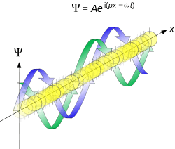
According to the de Broglie hypothesis, every object in the universe is a wave, i.e., a situation which gives rise to this phenomenon. The position of the particle is described by a wave function . The time-independent wave function of a single-moded plane wave of wavenumber k0 or momentum p0 is


The Born rule states that this should be interpreted as a probability density amplitude function in the sense that the probability of finding the particle between a and b is
![\operatorname {P} [a\leq X\leq b]=\int _{a}^{b}|\psi (x)|^{2}\,\mathrm {d} x~.](../I/m/f8852ff1f2e7c518fce8dfbb77f8e8a7920c63f3.svg)
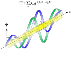
In the case of the single-moded plane wave, is a uniform distribution. In other words, the particle position is extremely uncertain in the sense that it could be essentially anywhere along the wave packet. Consider a wave function that is a sum of many waves, however, we may write this as


where An represents the relative contribution of the mode pn to the overall total. The figures to the right show how with the addition of many plane waves, the wave packet can become more localized. We may take this a step further to the continuum limit, where the wave function is an integral over all possible modes

with representing the amplitude of these modes and is called the wave function in momentum space. In mathematical terms, we say that is the Fourier transform of and that x and p are conjugate variables. Adding together all of these plane waves comes at a cost, namely the momentum has become less precise, having become a mixture of waves of many different momenta.


One way to quantify the precision of the position and momentum is the standard deviation σ. Since is a probability density function for position, we calculate its standard deviation.
The precision of the position is improved, i.e. reduced σx, by using many plane waves, thereby weakening the precision of the momentum, i.e. increased σp. Another way of stating this is that σx and σp have an inverse relationship or are at least bounded from below. This is the uncertainty principle, the exact limit of which is the Kennard bound. Click the show button below to see a semi-formal derivation of the Kennard inequality using wave mechanics.
| Proof of the Kennard inequality using wave mechanics |
|---|
| We are interested in the variances of position and momentum, defined as
Without loss of generality, we will assume that the means vanish, which just amounts to a shift of the origin of our coordinates. (A more general proof that does not make this assumption is given below.) This gives us the simpler form The function can be interpreted as a vector in a function space. We can define an inner product for a pair of functions u(x) and v(x) in this vector space: where the asterisk denotes the complex conjugate. With this inner product defined, we note that the variance for position can be written as We can repeat this for momentum by interpreting the function as a vector, but we can also take advantage of the fact that and are Fourier transforms of each other. We evaluate the inverse Fourier transform through integration by parts: where the canceled term vanishes because the wave function vanishes at infinity. Often the term is called the momentum operator in position space. Applying Parseval's theorem, we see that the variance for momentum can be written as The Cauchy–Schwarz inequality asserts that The modulus squared of any complex number z can be expressed as we let and and substitute these into the equation above to get All that remains is to evaluate these inner products. Plugging this into the above inequalities, we get or taking the square root Note that the only physics involved in this proof was that and are wave functions for position and momentum, which are Fourier transforms of each other. A similar result would hold for any pair of conjugate variables. |


![{\displaystyle {\begin{aligned}g(x)&={\frac {1}{\sqrt {2\pi \hbar }}}\cdot \int _{-\infty }^{\infty }{\tilde {g}}(p)\cdot e^{ipx/\hbar }\,dp\\&={\frac {1}{\sqrt {2\pi \hbar }}}\int _{-\infty }^{\infty }p\cdot \varphi (p)\cdot e^{ipx/\hbar }\,dp\\&={\frac {1}{2\pi \hbar }}\int _{-\infty }^{\infty }\left[p\cdot \int _{-\infty }^{\infty }\psi (\chi )e^{-ip\chi /\hbar }\,d\chi \right]\cdot e^{ipx/\hbar }\,dp\\&={\frac {i}{2\pi }}\int _{-\infty }^{\infty }\left[{\cancel {\left.\psi (\chi )e^{-ip\chi /\hbar }\right|_{-\infty }^{\infty }}}-\int _{-\infty }^{\infty }{\frac {d\psi (\chi )}{d\chi }}e^{-ip\chi /\hbar }\,d\chi \right]\cdot e^{ipx/\hbar }\,dp\\&={\frac {-i}{2\pi }}\int _{-\infty }^{\infty }\int _{-\infty }^{\infty }{\frac {d\psi (\chi )}{d\chi }}e^{-ip\chi /\hbar }\,d\chi \,e^{ipx/\hbar }\,dp\\&=\left(-i\hbar {\frac {d}{dx}}\right)\cdot \psi (x),\end{aligned}}}](../I/m/42db5a07d8c895b1e9caffa2cde0b6df608ec8f8.svg)


![{\displaystyle {\begin{aligned}\langle f\mid g\rangle -\langle g\mid f\rangle ={}&\int _{-\infty }^{\infty }\psi ^{*}(x)\,x\cdot \left(-i\hbar {\frac {d}{dx}}\right)\,\psi (x)\,dx\\&{}-\int _{-\infty }^{\infty }\psi ^{*}(x)\,\left(-i\hbar {\frac {d}{dx}}\right)\cdot x\,\psi (x)\,dx\\={}&i\hbar \cdot \int _{-\infty }^{\infty }\psi ^{*}(x)\left[\left(-x\cdot {\frac {d\psi (x)}{dx}}\right)+{\frac {d(x\psi (x))}{dx}}\right]\,dx\\={}&i\hbar \cdot \int _{-\infty }^{\infty }\psi ^{*}(x)\left[\left(-x\cdot {\frac {d\psi (x)}{dx}}\right)+\psi (x)+\left(x\cdot {\frac {d\psi (x)}{dx}}\right)\right]\,dx\\={}&i\hbar \cdot \int _{-\infty }^{\infty }\psi ^{*}(x)\psi (x)\,dx\\={}&i\hbar \cdot \int _{-\infty }^{\infty }|\psi (x)|^{2}\,dx\\={}&i\hbar \end{aligned}}}](../I/m/d4ddead3f7e2d237c2ad9bb5258ad66a9d92c599.svg)


Matrix mechanics interpretation
(Ref [10])
In matrix mechanics, observables such as position and momentum are represented by self-adjoint operators. When considering pairs of observables, an important quantity is the commutator. For a pair of operators  and B̂, one defines their commutator as
![[{\hat {A}},{\hat {B}}]={\hat {A}}{\hat {B}}-{\hat {B}}{\hat {A}}.](../I/m/3133da214f8f0fcf1ba11e907cfd121a2179b1b4.svg)
In the case of position and momentum, the commutator is the canonical commutation relation
![[{\hat {x}},{\hat {p}}]=i\hbar .](../I/m/fee0861ae7784cb51a1b43f6c51735c22c23274e.svg)
The physical meaning of the non-commutativity can be understood by considering the effect of the commutator on position and momentum eigenstates. Let be a right eigenstate of position with a constant eigenvalue x0. By definition, this means that Applying the commutator to yields


![{\displaystyle [{\hat {x}},{\hat {p}}]|\psi \rangle =({\hat {x}}{\hat {p}}-{\hat {p}}{\hat {x}})|\psi \rangle =({\hat {x}}-x_{0}{\hat {I}}){\hat {p}}\,|\psi \rangle =i\hbar |\psi \rangle ,}](../I/m/8255257353e4743e966c106dea5674689ed04690.svg)
where Î is the identity operator.
Suppose, for the sake of proof by contradiction, that is also a right eigenstate of momentum, with constant eigenvalue p0. If this were true, then one could write

On the other hand, the above canonical commutation relation requires that
![[{\hat {x}},{\hat {p}}]|\psi \rangle =i\hbar |\psi \rangle \neq 0.](../I/m/04d341bbd1c29d8f96a5ce5ad6e2cf856d1b1f40.svg)
This implies that no quantum state can simultaneously be both a position and a momentum eigenstate.
When a state is measured, it is projected onto an eigenstate in the basis of the relevant observable. For example, if a particle's position is measured, then the state amounts to a position eigenstate. This means that the state is not a momentum eigenstate, however, but rather it can be represented as a sum of multiple momentum basis eigenstates. In other words, the momentum must be less precise. This precision may be quantified by the standard deviations,


As in the wave mechanics interpretation above, one sees a tradeoff between the respective precisions of the two, quantified by the uncertainty principle.
Robertson–Schrödinger uncertainty relations
The most common general form of the uncertainty principle is the Robertson uncertainty relation.[17]
For an arbitrary Hermitian operator we can associate a standard deviation


where the brackets indicate an expectation value. For a pair of operators and , we may define their commutator as


![[\hat{A},\hat{B}]=\hat{A}\hat{B}-\hat{B}\hat{A},](../I/m/9814a77ea436e956fd7abaad7b5906457037b565.svg)
In this notation, the Robertson uncertainty relation is given by
![{\displaystyle \sigma _{A}\sigma _{B}\geq \left|{\frac {1}{2i}}\langle [{\hat {A}},{\hat {B}}]\rangle \right|={\frac {1}{2}}\left|\langle [{\hat {A}},{\hat {B}}]\rangle \right|,}](../I/m/2e237cc47d6a6ffaf614f696672356c362f84ac0.svg)
The Robertson uncertainty relation immediately follows from a slightly stronger inequality, the Schrödinger uncertainty relation,[18]
![{\displaystyle \sigma _{A}^{2}\sigma _{B}^{2}\geq \left|{\frac {1}{2}}\langle \{{\hat {A}},{\hat {B}}\}\rangle -\langle {\hat {A}}\rangle \langle {\hat {B}}\rangle \right|^{2}+\left|{\frac {1}{2i}}\langle [{\hat {A}},{\hat {B}}]\rangle \right|^{2},}](../I/m/81d7a893fe43757553fb6a3e5a51cdb83290aadd.svg)
where we have introduced the anticommutator,

| Proof of the Schrödinger uncertainty relation | ||||||||||||||||||||||||||||
|---|---|---|---|---|---|---|---|---|---|---|---|---|---|---|---|---|---|---|---|---|---|---|---|---|---|---|---|---|
| The derivation shown here incorporates and builds off of those shown in Robertson,[17] Schrödinger[18] and standard textbooks such as Griffiths.[19] For any Hermitian operator
, based upon the definition of variance, we have
we let and thus Similarly, for any other Hermitian operator in the same state for The product of the two deviations can thus be expressed as
In order to relate the two vectors and , we use the Cauchy–Schwarz inequality[20] which is defined as and thus Eq. (1) can be written as
Since is in general a complex number, we use the fact that the modulus squared of any complex number is defined as , where is the complex conjugate of . The modulus squared can also be expressed as
we let and and substitute these into the equation above to get
The inner product is written out explicitly as and using the fact that and are Hermitian operators, we find Similarly it can be shown that Thus we have and We now substitute the above two equations above back into Eq. (4) and get Substituting the above into Eq. (2) we get the Schrödinger uncertainty relation This proof has an issue[21] related to the domains of the operators involved. For the proof to make sense, the vector has to be in the domain of the unbounded operator , which is not always the case. In fact, the Robertson uncertainty relation is false if is an angle variable and is the derivative with respect to this variable. In this example, the commutator is a nonzero constant—just as in the Heisenberg uncertainty relation—and yet there are states where the product of the uncertainties is zero.[22] (See the counterexample section below.) This issue can be overcome by using a variational method for the proof.,[23][24] or by working with an exponentiated version of the canonical commutation relations.[22] Note that in the general form of the Robertson–Schrödinger uncertainty relation, there is no need to assume that the operators and are self-adjoint operators. It suffices to assume that they are merely symmetric operators. (The distinction between these two notions is generally glossed over in the physics literature, where the term Hermitian is used for either or both classes of operators. See Chapter 9 of Hall's book[25] for a detailed discussion of this important but technical distinction.) |


![{\displaystyle {\begin{aligned}\langle f\mid g\rangle &=\langle \Psi |({\hat {A}}-\langle {\hat {A}}\rangle )({\hat {B}}-\langle {\hat {B}}\rangle )\Psi \rangle \\[4pt]&=\langle \Psi \mid ({\hat {A}}{\hat {B}}-{\hat {A}}\langle {\hat {B}}\rangle -{\hat {B}}\langle {\hat {A}}\rangle +\langle {\hat {A}}\rangle \langle {\hat {B}}\rangle )\Psi \rangle \\[4pt]&=\langle \Psi \mid {\hat {A}}{\hat {B}}\Psi \rangle -\langle \Psi \mid {\hat {A}}\langle {\hat {B}}\rangle \Psi \rangle -\langle \Psi \mid {\hat {B}}\langle {\hat {A}}\rangle \Psi \rangle +\langle \Psi \mid \langle {\hat {A}}\rangle \langle {\hat {B}}\rangle \Psi \rangle \\[4pt]&=\langle {\hat {A}}{\hat {B}}\rangle -\langle {\hat {A}}\rangle \langle {\hat {B}}\rangle -\langle {\hat {A}}\rangle \langle {\hat {B}}\rangle +\langle {\hat {A}}\rangle \langle {\hat {B}}\rangle \\[4pt]&=\langle {\hat {A}}{\hat {B}}\rangle -\langle {\hat {A}}\rangle \langle {\hat {B}}\rangle .\end{aligned}}}](../I/m/e8c0c05428ab53be785878d1546c265c45c6e755.svg)

![{\displaystyle \langle f\mid g\rangle -\langle g\mid f\rangle =\langle {\hat {A}}{\hat {B}}\rangle -\langle {\hat {A}}\rangle \langle {\hat {B}}\rangle -\langle {\hat {B}}{\hat {A}}\rangle +\langle {\hat {A}}\rangle \langle {\hat {B}}\rangle =\langle [{\hat {A}},{\hat {B}}]\rangle }](../I/m/eaf12a5caf8e73c4e1cfdfbbf3ebb1c3e32e7e0f.svg)

![{\displaystyle |\langle f\mid g\rangle |^{2}={\Big (}{\frac {1}{2}}\langle \{{\hat {A}},{\hat {B}}\}\rangle -\langle {\hat {A}}\rangle \langle {\hat {B}}\rangle {\Big )}^{2}+{\Big (}{\frac {1}{2i}}\langle [{\hat {A}},{\hat {B}}]\rangle {\Big )}^{2}\,.}](../I/m/074cd206c3b6789fd747fa2efa892ea596651470.svg)
![{\displaystyle \sigma _{A}\sigma _{B}\geq {\sqrt {{\Big (}{\frac {1}{2}}\langle \{{\hat {A}},{\hat {B}}\}\rangle -\langle {\hat {A}}\rangle \langle {\hat {B}}\rangle {\Big )}^{2}+{\Big (}{\frac {1}{2i}}\langle [{\hat {A}},{\hat {B}}]\rangle {\Big )}^{2}}}.}](../I/m/96a2a724edaa3e9b3e175f7de8158b796bef58c0.svg)

Examples
Since the Robertson and Schrödinger relations are for general operators, the relations can be applied to any two observables to obtain specific uncertainty relations. A few of the most common relations found in the literature are given below.
- For position and linear momentum, the canonical commutation relation implies the Kennard inequality from above:
![{\displaystyle [{\hat {x}},{\hat {p}}]=i\hbar }](../I/m/42dbbd0db710385288536bcf4f4a1b7cceb75d9a.svg)

- For two orthogonal components of the total angular momentum operator of an object:
- where i, j, k are distinct, and Ji denotes angular momentum along the xi axis. This relation implies that unless all three components vanish together, only a single component of a system's angular momentum can be defined with arbitrary precision, normally the component parallel to an external (magnetic or electric) field. Moreover, for , a choice , , in angular momentum multiplets, ψ = |j, m〉, bounds the Casimir invariant (angular momentum squared, ) from below and thus yields useful constraints such as j(j + 1) ≥ m(m + 1), and hence j ≥ m, among others.

![{\displaystyle [J_{x},J_{y}]=i\hbar \varepsilon _{xyz}J_{z}}](../I/m/92feb40a1e1bb732beffa55c687ccfbcec8ff007.svg)


- In non-relativistic mechanics, time is privileged as an independent variable. Nevertheless, in 1945, L. I. Mandelshtam and I. E. Tamm derived a non-relativistic time–energy uncertainty relation, as follows.[26][27] For a quantum system in a non-stationary state ψ and an observable B represented by a self-adjoint operator , the following formula holds:
- where σE is the standard deviation of the energy operator (Hamiltonian) in the state ψ, σB stands for the standard deviation of B. Although the second factor in the left-hand side has dimension of time, it is different from the time parameter that enters the Schrödinger equation. It is a lifetime of the state ψ with respect to the observable B: In other words, this is the time interval (Δt) after which the expectation value changes appreciably.
- An informal, heuristic meaning of the principle is the following: A state that only exists for a short time cannot have a definite energy. To have a definite energy, the frequency of the state must be defined accurately, and this requires the state to hang around for many cycles, the reciprocal of the required accuracy. For example, in spectroscopy, excited states have a finite lifetime. By the time–energy uncertainty principle, they do not have a definite energy, and, each time they decay, the energy they release is slightly different. The average energy of the outgoing photon has a peak at the theoretical energy of the state, but the distribution has a finite width called the natural linewidth. Fast-decaying states have a broad linewidth, while slow-decaying states have a narrow linewidth.[28]
- The same linewidth effect also makes it difficult to specify the rest mass of unstable, fast-decaying particles in particle physics. The faster the particle decays (the shorter its lifetime), the less certain is its mass (the larger the particle's width).


- For the number of electrons in a superconductor and the phase of its Ginzburg–Landau order parameter[29][30]

A counterexample
Suppose we consider a quantum particle on a ring, where the wave function depends on an angular variable , which we may take to lie in the interval . Define "position" and "momentum" operators and by

![[0,2\pi]](../I/m/348d40bf3f8b7e1c00c4346440d7e2e4f0cc9b91.svg)
![{\displaystyle {\hat {A}}\psi (\theta )=\theta \psi (\theta ),\quad \theta \in [0,2\pi ],}](../I/m/f85b2a63d69030bd4deabafe7641563413b8ec23.svg)
and

where we impose periodic boundary conditions on . Note that the definition of depends on our choice to have range from 0 to . These operators satisfy the usual commutation relations for position and momentum operators, .[31]

![{\displaystyle [{\hat {A}},{\hat {B}}]=i\hbar }](../I/m/ac8c6748f07eed66c5b329fcebdb8ca9d859ff71.svg)
Now let be any of the eigenstates of , which are given by . Note that these states are normalizable, unlike the eigenstates of the momentum operator on the line. Note also that the operator is bounded, since ranges over a bounded interval. Thus, in the state , the uncertainty of is zero and the uncertainty of is finite, so that


Although this result appears to violate the Robertson uncertainty principle, the paradox is resolved when we note that is not in the domain of the operator , since multiplication by disrupts the periodic boundary conditions imposed on .[22] Thus, the derivation of the Robertson relation, which requires and to be defined, does not apply. (These also furnish an example of operators satisfying the canonical commutation relations but not the Weyl relations.[32])


For the usual position and momentum operators and on the real line, no such counterexamples can occur. As long as and are defined in the state , the Heisenberg uncertainty principle holds, even if fails to be in the domain of or of .[33]


Examples
Quantum harmonic oscillator stationary states
Consider a one-dimensional quantum harmonic oscillator (QHO). It is possible to express the position and momentum operators in terms of the creation and annihilation operators:


Using the standard rules for creation and annihilation operators on the eigenstates of the QHO,


the variances may be computed directly,


The product of these standard deviations is then

In particular, the above Kennard bound[3] is saturated for the ground state n=0, for which the probability density is just the normal distribution.
Quantum harmonic oscillator with Gaussian initial condition
In a quantum harmonic oscillator of characteristic angular frequency ω, place a state that is offset from the bottom of the potential by some displacement x0 as

where Ω describes the width of the initial state but need not be the same as ω. Through integration over the propagator, we can solve for the full time-dependent solution. After many cancelations, the probability densities reduce to


where we have used the notation to denote a normal distribution of mean μ and variance σ2. Copying the variances above and applying trigonometric identities, we can write the product of the standard deviations as


From the relations

we can conclude the following: (the right most equality holds only when Ω = ω) .

Coherent states
A coherent state is a right eigenstate of the annihilation operator,
- ,

which may be represented in terms of Fock states as

In the picture where the coherent state is a massive particle in a QHO, the position and momentum operators may be expressed in terms of the annihilation operators in the same formulas above and used to calculate the variances,


Therefore, every coherent state saturates the Kennard bound

with position and momentum each contributing an amount in a "balanced" way. Moreover, every squeezed coherent state also saturates the Kennard bound although the individual contributions of position and momentum need not be balanced in general.

Particle in a box
Consider a particle in a one-dimensional box of length . The eigenfunctions in position and momentum space are


and

where and we have used the de Broglie relation . The variances of and can be calculated explicitly:


The product of the standard deviations is therefore

For all , the quantity is greater than 1, so the uncertainty principle is never violated. For numerical concreteness, the smallest value occurs when , in which case


Constant momentum
Assume a particle initially has a momentum space wave function described by a normal distribution around some constant momentum p0 according to

where we have introduced a reference scale , with describing the width of the distribution−−cf. nondimensionalization. If the state is allowed to evolve in free space, then the time-dependent momentum and position space wave functions are


Since and this can be interpreted as a particle moving along with constant momentum at arbitrarily high precision. On the other hand, the standard deviation of the position is


such that the uncertainty product can only increase with time as

Additional uncertainty relations
Mixed states
The Robertson–Schrödinger uncertainty relation may be generalized in a straightforward way to describe mixed states.[34]
![{\displaystyle \sigma _{A}^{2}\sigma _{B}^{2}\geq \left({\frac {1}{2}}\operatorname {tr} (\rho \{A,B\})-\operatorname {tr} (\rho A)\operatorname {tr} (\rho B)\right)^{2}+\left({\frac {1}{2i}}\operatorname {tr} (\rho [A,B])\right)^{2}}](../I/m/ede80f166400229a6ce137edbeb825f4178c3733.svg)
The Maccone–Pati uncertainty relations
The Robertson–Schrödinger uncertainty relation can be trivial if the state of the system is chosen to be eigenstate of one of the observable. The stronger uncertainty relations proved by Maccone and Pati give non-trivial bounds on the sum of the variances for two incompatible observables.[35] For two non-commuting observables and the first stronger uncertainty relation is given by
![{\displaystyle \sigma _{A}^{2}+\sigma _{B}^{2}\geq \pm i\langle \Psi \mid [A,B]|\Psi \rangle +\mid \langle \Psi \mid (A\pm iB)\mid {\bar {\Psi }}\rangle |^{2},}](../I/m/fe87035b4463c5578ccda71d74b8e7c9fd627515.svg)
where , , is a normalized vector that is orthogonal to the state of the system and one should choose the sign of to make this real quantity a positive number.


![{\displaystyle \pm i\langle \Psi \mid [A,B]\mid \Psi \rangle }](../I/m/3a34a5250780e2a23b4befafff39d5522cc8266c.svg)
The second stronger uncertainty relation is given by

where is a state orthogonal to . The form of implies that the right-hand side of the new uncertainty relation is nonzero unless is an eigenstate of . One may note that can be an eigenstate of without being an eigenstate of either or . However, when is an eigenstate of one of the two observables the Heisenberg–Schrödinger uncertainty relation becomes trivial. But the lower bound in the new relation is nonzero unless is an eigenstate of both.


Phase space
In the phase space formulation of quantum mechanics, the Robertson–Schrödinger relation follows from a positivity condition on a real star-square function. Given a Wigner function with star product ★ and a function f, the following is generally true:[36]


Choosing , we arrive at


Since this positivity condition is true for all a, b, and c, it follows that all the eigenvalues of the matrix are positive. The positive eigenvalues then imply a corresponding positivity condition on the determinant:

or, explicitly, after algebraic manipulation,

Systematic and statistical errors
The inequalities above focus on the statistical imprecision of observables as quantified by the standard deviation . Heisenberg's original version, however, was dealing with the systematic error, a disturbance of the quantum system produced by the measuring apparatus, i.e., an observer effect.

If we let represent the error (i.e., inaccuracy) of a measurement of an observable A and the disturbance produced on a subsequent measurement of the conjugate variable B by the former measurement of A, then the inequality proposed by Ozawa[6] — encompassing both systematic and statistical errors — holds:


![{\displaystyle \varepsilon _{A}\,\eta _{B}+\varepsilon _{A}\,\sigma _{B}+\sigma _{A}\,\eta _{B}\,\geq \,{\frac {1}{2}}\,\left|\langle [{\hat {A}},{\hat {B}}]\rangle \right|}](../I/m/507c66d05ec579594d36bbca8d92a3d2591a3145.svg)
Heisenberg's uncertainty principle, as originally described in the 1927 formulation, mentions only the first term of Ozawa inequality, regarding the systematic error. Using the notation above to describe the error/disturbance effect of sequential measurements (first A, then B), it could be written as
![{\displaystyle \varepsilon _{A}\,\eta _{B}\,\geq \,{\frac {1}{2}}\,\left|\langle [{\hat {A}},{\hat {B}}]\rangle \right|}](../I/m/1c0ac9415761d7b6ee02cba76450b3f36cc5568d.svg)
The formal derivation of the Heisenberg relation is possible but far from intuitive. It was not proposed by Heisenberg, but formulated in a mathematically consistent way only in recent years.[37][38] Also, it must be stressed that the Heisenberg formulation is not taking into account the intrinsic statistical errors and . There is increasing experimental evidence[8][39][40][41] that the total quantum uncertainty cannot be described by the Heisenberg term alone, but requires the presence of all the three terms of the Ozawa inequality.


Using the same formalism,[1] it is also possible to introduce the other kind of physical situation, often confused with the previous one, namely the case of simultaneous measurements (A and B at the same time):
![{\displaystyle \varepsilon _{A}\,\varepsilon _{B}\,\geq \,{\frac {1}{2}}\,\left|\langle [{\hat {A}},{\hat {B}}]\rangle \right|}](../I/m/c40783a21b640620ef335dca2937ee9ac7aa9a50.svg)
The two simultaneous measurements on A and B are necessarily[42] unsharp or weak.
It is also possible to derive an uncertainty relation that, as the Ozawa's one, combines both the statistical and systematic error components, but keeps a form very close to the Heisenberg original inequality. By adding Robertson[1]
![{\displaystyle \sigma _{A}\,\sigma _{B}\,\geq \,{\frac {1}{2}}\,\left|\langle [{\hat {A}},{\hat {B}}]\rangle \right|}](../I/m/459f27fa54d560f33387b243214030b31e08d12b.svg)
and Ozawa relations we obtain
![{\displaystyle \varepsilon _{A}\eta _{B}+\varepsilon _{A}\,\sigma _{B}+\sigma _{A}\,\eta _{B}+\sigma _{A}\sigma _{B}\geq \left|\langle [{\hat {A}},{\hat {B}}]\rangle \right|.}](../I/m/1dc1e7900ca212f157f381dda5fea49f2885ff78.svg)
The four terms can be written as:
![{\displaystyle (\varepsilon _{A}+\sigma _{A})\,(\eta _{B}+\sigma _{B})\,\geq \,\left|\langle [{\hat {A}},{\hat {B}}]\rangle \right|.}](../I/m/308a2567453272bef9b35660c39ab39513051e56.svg)
Defining:

as the inaccuracy in the measured values of the variable A and

as the resulting fluctuation in the conjugate variable B, Fujikawa[43] established an uncertainty relation similar to the Heisenberg original one, but valid both for systematic and statistical errors:
![{\displaystyle {\bar {\varepsilon }}_{A}\,{\bar {\eta }}_{B}\,\geq \,\left|\langle [{\hat {A}},{\hat {B}}]\rangle \right|}](../I/m/2e6fd7cd1c81287fb8d7f07f732dd943c30114e7.svg)
Quantum entropic uncertainty principle
For many distributions, the standard deviation is not a particularly natural way of quantifying the structure. For example, uncertainty relations in which one of the observables is an angle has little physical meaning for fluctuations larger than one period.[24][44][45][46] Other examples include highly bimodal distributions, or unimodal distributions with divergent variance.
A solution that overcomes these issues is an uncertainty based on entropic uncertainty instead of the product of variances. While formulating the many-worlds interpretation of quantum mechanics in 1957, Hugh Everett III conjectured a stronger extension of the uncertainty principle based on entropic certainty.[47] This conjecture, also studied by Hirschman[48] and proven in 1975 by Beckner[49] and by Iwo Bialynicki-Birula and Jerzy Mycielski[50] is that, for two normalized, dimensionless Fourier transform pairs f(a) and g(b) where
- and


the Shannon information entropies

and

are subject to the following constraint,

where the logarithms may be in any base.
The probability distribution functions associated with the position wave function ψ(x) and the momentum wave function φ(x) have dimensions of inverse length and momentum respectively, but the entropies may be rendered dimensionless by


where x0 and p0 are some arbitrarily chosen length and momentum respectively, which render the arguments of the logarithms dimensionless. Note that the entropies will be functions of these chosen parameters. Due to the Fourier transform relation between the position wave function ψ(x) and the momentum wavefunction φ(p), the above constraint can be written for the corresponding entropies as

where h is Planck's constant.
Depending on one's choice of the x0 p0 product, the expression may be written in many ways. If x0 p0 is chosen to be h, then

If, instead, x0 p0 is chosen to be ħ, then

If x0 and p0 are chosen to be unity in whatever system of units are being used, then

where h is interpreted as a dimensionless number equal to the value of Planck's constant in the chosen system of units.
The quantum entropic uncertainty principle is more restrictive than the Heisenberg uncertainty principle. From the inverse logarithmic Sobolev inequalities[51]


(equivalently, from the fact that normal distributions maximize the entropy of all such with a given variance), it readily follows that this entropic uncertainty principle is stronger than the one based on standard deviations, because

In other words, the Heisenberg uncertainty principle, is a consequence of the quantum entropic uncertainty principle, but not vice versa. A few remarks on these inequalities. First, the choice of base e is a matter of popular convention in physics. The logarithm can alternatively be in any base, provided that it be consistent on both sides of the inequality. Second, recall the Shannon entropy has been used, not the quantum von Neumann entropy. Finally, the normal distribution saturates the inequality, and it is the only distribution with this property, because it is the maximum entropy probability distribution among those with fixed variance (cf. here for proof).
| Entropic uncertainty of the normal distribution |
|---|
| We demonstrate this method on the ground state of the QHO, which as discussed above saturates the usual uncertainty based on standard deviations. The length scale can be set to whatever is convenient, so we assign
The probability distribution is the normal distribution with Shannon entropy A completely analogous calculation proceeds for the momentum distribution. Choosing a standard momentum of : The entropic uncertainty is therefore the limiting value |


![{\displaystyle {\begin{aligned}H_{x}&=-\int |\psi (x)|^{2}\ln(|\psi (x)|^{2}\cdot x_{0})\,dx\\&=-{\frac {1}{x_{0}{\sqrt {2\pi }}}}\int _{-\infty }^{\infty }\exp {\left(-{\frac {x^{2}}{2x_{0}^{2}}}\right)}\ln \left[{\frac {1}{\sqrt {2\pi }}}\exp {\left(-{\frac {x^{2}}{2x_{0}^{2}}}\right)}\right]\,dx\\&={\frac {1}{\sqrt {2\pi }}}\int _{-\infty }^{\infty }\exp {\left(-{\frac {u^{2}}{2}}\right)}\left[\ln({\sqrt {2\pi }})+{\frac {u^{2}}{2}}\right]\,du\\&=\ln({\sqrt {2\pi }})+{\frac {1}{2}}.\end{aligned}}}](../I/m/124b7c9778e717ecae5fb23df17a3e6ea1cdab89.svg)


![{\displaystyle {\begin{aligned}H_{p}&=-\int |\varphi (p)|^{2}\ln(|\varphi (p)|^{2}\cdot \hbar /x_{0})\,dp\\&=-{\sqrt {\frac {2x_{0}^{2}}{\pi \hbar ^{2}}}}\int _{-\infty }^{\infty }\exp {\left(-{\frac {2x_{0}^{2}p^{2}}{\hbar ^{2}}}\right)}\ln \left[{\sqrt {\frac {2}{\pi }}}\exp {\left(-{\frac {2x_{0}^{2}p^{2}}{\hbar ^{2}}}\right)}\right]\,dp\\&={\sqrt {\frac {2}{\pi }}}\int _{-\infty }^{\infty }\exp {\left(-2v^{2}\right)}\left[\ln \left({\sqrt {\frac {\pi }{2}}}\right)+2v^{2}\right]\,dv\\&=\ln \left({\sqrt {\frac {\pi }{2}}}\right)+{\frac {1}{2}}.\end{aligned}}}](../I/m/8106bc906d97851869d4000e4d3d0dd8e7916e56.svg)

A measurement apparatus will have a finite resolution set by the discretization of its possible outputs into bins, with the probability of lying within one of the bins given by the Born rule. We will consider the most common experimental situation, in which the bins are of uniform size. Let δx be a measure of the spatial resolution. We take the zeroth bin to be centered near the origin, with possibly some small constant offset c. The probability of lying within the jth interval of width δx is
![{\displaystyle \operatorname {P} [x_{j}]=\int _{(j-1/2)\delta x-c}^{(j+1/2)\delta x-c}|\psi (x)|^{2}\,dx}](../I/m/b7c173529c81593fd8c2e56a4e1af15f369c365c.svg)
To account for this discretization, we can define the Shannon entropy of the wave function for a given measurement apparatus as
![{\displaystyle H_{x}=-\sum _{j=-\infty }^{\infty }\operatorname {P} [x_{j}]\ln \operatorname {P} [x_{j}].}](../I/m/25c2fd9ede05e0615e6eff1a8f2ace626debd818.svg)
Under the above definition, the entropic uncertainty relation is

Here we note that δx δp/h is a typical infinitesimal phase space volume used in the calculation of a partition function. The inequality is also strict and not saturated. Efforts to improve this bound are an active area of research.
| Normal distribution example |
|---|
| We demonstrate this method first on the ground state of the QHO, which as discussed above saturates the usual uncertainty based on standard deviations.
The probability of lying within one of these bins can be expressed in terms of the error function. The momentum probabilities are completely analogous. For simplicity, we will set the resolutions to so that the probabilities reduce to The Shannon entropy can be evaluated numerically. The entropic uncertainty is indeed larger than the limiting value. Note that despite being in the optimal case, the inequality is not saturated. |

![{\displaystyle {\begin{aligned}\operatorname {P} [x_{j}]&={\sqrt {\frac {m\omega }{\pi \hbar }}}\int _{(j-1/2)\delta x}^{(j+1/2)\delta x}\exp \left(-{\frac {m\omega x^{2}}{\hbar }}\right)\,dx\\&={\sqrt {\frac {1}{\pi }}}\int _{(j-1/2)\delta x{\sqrt {m\omega /\hbar }}}^{(j+1/2)\delta x{\sqrt {m\omega /\hbar }}}e^{u^{2}}\,du\\&={\frac {1}{2}}\left[\operatorname {erf} \left(\left(j+{\frac {1}{2}}\right)\delta x\cdot {\sqrt {\frac {m\omega }{\hbar }}}\right)-\operatorname {erf} \left(\left(j-{\frac {1}{2}}\right)\delta x\cdot {\sqrt {\frac {m\omega }{\hbar }}}\right)\right]\end{aligned}}}](../I/m/fb98a69e46b2d10143459959d1679c78443b6378.svg)
![{\displaystyle \operatorname {P} [p_{j}]={\frac {1}{2}}\left[\operatorname {erf} \left(\left(j+{\frac {1}{2}}\right)\delta p\cdot {\frac {1}{\sqrt {\hbar m\omega }}}\right)-\operatorname {erf} \left(\left(j-{\frac {1}{2}}\right)\delta x\cdot {\frac {1}{\sqrt {\hbar m\omega }}}\right)\right]}](../I/m/ed784fa900105bac03e1163a54fc3dd5732367aa.svg)


![{\displaystyle \operatorname {P} [x_{j}]=\operatorname {P} [p_{j}]={\frac {1}{2}}\left[\operatorname {erf} \left(\left(j+{\frac {1}{2}}\right){\sqrt {2\pi }}\right)-\operatorname {erf} \left(\left(j-{\frac {1}{2}}\right){\sqrt {2\pi }}\right)\right]}](../I/m/ba65e2143152330bf233c24e6524ac16a365c168.svg)
![{\displaystyle {\begin{aligned}H_{x}=H_{p}&=-\sum _{j=-\infty }^{\infty }\operatorname {P} [x_{j}]\ln \operatorname {P} [x_{j}]\\&=-\sum _{j=-\infty }^{\infty }{\frac {1}{2}}\left[\operatorname {erf} \left(\left(j+{\frac {1}{2}}\right){\sqrt {2\pi }}\right)-\operatorname {erf} \left(\left(j-{\frac {1}{2}}\right){\sqrt {2\pi }}\right)\right]\ln {\frac {1}{2}}\left[\operatorname {erf} \left(\left(j+{\frac {1}{2}}\right){\sqrt {2\pi }}\right)-\operatorname {erf} \left(\left(j-{\frac {1}{2}}\right){\sqrt {2\pi }}\right)\right]&\approx 0.3226\end{aligned}}}](../I/m/7edfbe77762479a164b5863aa0f72ef098e1df08.svg)

| Sinc function example |
|---|
| An example of a unimodal distribution with infinite variance is the sinc function. If the wave function is the correctly normalized uniform distribution,
then its Fourier transform is the sinc function, which yields infinite momentum variance despite having a centralized shape. The entropic uncertainty, on the other hand, is finite. Suppose for simplicity that the spatial resolution is just a two-bin measurement, δx = a, and that the momentum resolution is δp = h/a. Partitioning the uniform spatial distribution into two equal bins is straightforward. We set the offset c = 1/2 so that the two bins span the distribution. The bins for momentum must cover the entire real line. As done with the spatial distribution, we could apply an offset. It turns out, however, that the Shannon entropy is minimized when the zeroth bin for momentum is centered at the origin. (The reader is encouraged to try adding an offset.) The probability of lying within an arbitrary momentum bin can be expressed in terms of the sine integral. The Shannon entropy can be evaluated numerically. The entropic uncertainty is indeed larger than the limiting value. |
![{\displaystyle \psi (x)={\begin{cases}{\frac {1}{\sqrt {2a}}}&{\text{for }}|x|\leq a,\\[8pt]0&{\text{for }}|x|>a\end{cases}}}](../I/m/ea3f0b2acef217f888c5fe38d2985169b925da48.svg)

![{\displaystyle \operatorname {P} [x_{0}]=\int _{-a}^{0}{\frac {1}{2a}}\,dx={\frac {1}{2}}}](../I/m/4bb8e8e07cba14e44ac3fd1f812c87b344f79978.svg)
![{\displaystyle \operatorname {P} [x_{1}]=\int _{0}^{a}{\frac {1}{2a}}\,dx={\frac {1}{2}}}](../I/m/abb619286fac29cd04fb8ad539e4d7fc979da3fd.svg)
![{\displaystyle H_{x}=-\sum _{j=0}^{1}\operatorname {P} [x_{j}]\ln \operatorname {P} [x_{j}]=-{\frac {1}{2}}\ln {\frac {1}{2}}-{\frac {1}{2}}\ln {\frac {1}{2}}=\ln 2}](../I/m/fd49a257fd5578026bd28e8e539dccfaae24dd1f.svg)
![{\displaystyle {\begin{aligned}\operatorname {P} [p_{j}]&={\frac {a}{\pi \hbar }}\int _{(j-1/2)\delta p}^{(j+1/2)\delta p}\operatorname {sinc} ^{2}\left({\frac {ap}{\hbar }}\right)\,dp\\&={\frac {1}{\pi }}\int _{2\pi (j-1/2)}^{2\pi (j+1/2)}\operatorname {sinc} ^{2}(u)\,du\\&={\frac {1}{\pi }}\left[\operatorname {Si} ((4j+2)\pi )-\operatorname {Si} ((4j-2)\pi )\right]\end{aligned}}}](../I/m/4c11b911bee6171d2a7ac1ee1c5522d49625ffb2.svg)
![{\displaystyle H_{p}=-\sum _{j=-\infty }^{\infty }\operatorname {P} [p_{j}]\ln \operatorname {P} [p_{j}]=-\operatorname {P} [p_{0}]\ln \operatorname {P} [p_{0}]-2\cdot \sum _{j=1}^{\infty }\operatorname {P} [p_{j}]\ln \operatorname {P} [p_{j}]\approx 0.53}](../I/m/ae44da862dea854275b063fc3b5fe01bd3f3309f.svg)

Harmonic analysis
In the context of harmonic analysis, a branch of mathematics, the uncertainty principle implies that one cannot at the same time localize the value of a function and its Fourier transform. To wit, the following inequality holds,

Further mathematical uncertainty inequalities, including the above entropic uncertainty, hold between a function f and its Fourier transform ƒ̂:[52][53][54]

Signal processing
In the context of signal processing, and in particular time–frequency analysis, uncertainty principles are referred to as the Gabor limit, after Dennis Gabor, or sometimes the Heisenberg–Gabor limit. The basic result, which follows from "Benedicks's theorem", below, is that a function cannot be both time limited and band limited (a function and its Fourier transform cannot both have bounded domain)—see bandlimited versus timelimited. Thus

where and are the standard deviations of the time and frequency estimates respectively [55].


Stated alternatively, "One cannot simultaneously sharply localize a signal (function f ) in both the time domain and frequency domain ( ƒ̂, its Fourier transform)".
When applied to filters, the result implies that one cannot achieve high temporal resolution and frequency resolution at the same time; a concrete example are the resolution issues of the short-time Fourier transform—if one uses a wide window, one achieves good frequency resolution at the cost of temporal resolution, while a narrow window has the opposite trade-off.
Alternate theorems give more precise quantitative results, and, in time–frequency analysis, rather than interpreting the (1-dimensional) time and frequency domains separately, one instead interprets the limit as a lower limit on the support of a function in the (2-dimensional) time–frequency plane. In practice, the Gabor limit limits the simultaneous time–frequency resolution one can achieve without interference; it is possible to achieve higher resolution, but at the cost of different components of the signal interfering with each other.
DFT-Uncertainty principle
There is an uncertainty principle that uses signal sparsity (or the number of non-zero coefficients).[56]
Let be a sequence of N complex numbers and its discrete Fourier transform.


Denote by the number of non-zero elements in the time sequence and by the number of non-zero elements in the frequency sequence . Then,


Benedicks's theorem
Amrein–Berthier[57] and Benedicks's theorem[58] intuitively says that the set of points where f is non-zero and the set of points where ƒ̂ is non-zero cannot both be small.
Specifically, it is impossible for a function f in L2(R) and its Fourier transform ƒ̂ to both be supported on sets of finite Lebesgue measure. A more quantitative version is[59][60]

One expects that the factor CeC|S||Σ| may be replaced by CeC(|S||Σ|)1/d, which is only known if either S or Σ is convex.
Hardy's uncertainty principle
The mathematician G. H. Hardy formulated the following uncertainty principle:[61] it is not possible for f and ƒ̂ to both be "very rapidly decreasing". Specifically, if f in L2(R) is such that

and
- ( an integer),


then, if ab > 1, f = 0, while if ab = 1, then there is a polynomial P of degree ≤ N such that

This was later improved as follows: if f ∈ L2(Rd) is such that

then

where P is a polynomial of degree (N − d)/2 and A is a real d×d positive definite matrix.
This result was stated in Beurling's complete works without proof and proved in Hörmander[62] (the case ) and Bonami, Demange, and Jaming[63] for the general case. Note that Hörmander–Beurling's version implies the case ab > 1 in Hardy's Theorem while the version by Bonami–Demange–Jaming covers the full strength of Hardy's Theorem. A different proof of Beurling's theorem based on Liouville's theorem appeared in ref.[64]

A full description of the case ab < 1 as well as the following extension to Schwartz class distributions appears in ref.[65]
Theorem. If a tempered distribution is such that


and

then
for some convenient polynomial P and real positive definite matrix A of type d × d.
History
Werner Heisenberg formulated the uncertainty principle at Niels Bohr's institute in Copenhagen, while working on the mathematical foundations of quantum mechanics.[66]
In 1925, following pioneering work with Hendrik Kramers, Heisenberg developed matrix mechanics, which replaced the ad hoc old quantum theory with modern quantum mechanics. The central premise was that the classical concept of motion does not fit at the quantum level, as electrons in an atom do not travel on sharply defined orbits. Rather, their motion is smeared out in a strange way: the Fourier transform of its time dependence only involves those frequencies that could be observed in the quantum jumps of their radiation.
Heisenberg's paper did not admit any unobservable quantities like the exact position of the electron in an orbit at any time; he only allowed the theorist to talk about the Fourier components of the motion. Since the Fourier components were not defined at the classical frequencies, they could not be used to construct an exact trajectory, so that the formalism could not answer certain overly precise questions about where the electron was or how fast it was going.
In March 1926, working in Bohr's institute, Heisenberg realized that the non-commutativity implies the uncertainty principle. This implication provided a clear physical interpretation for the non-commutativity, and it laid the foundation for what became known as the Copenhagen interpretation of quantum mechanics. Heisenberg showed that the commutation relation implies an uncertainty, or in Bohr's language a complementarity.[67] Any two variables that do not commute cannot be measured simultaneously—the more precisely one is known, the less precisely the other can be known. Heisenberg wrote:
It can be expressed in its simplest form as follows: One can never know with perfect accuracy both of those two important factors which determine the movement of one of the smallest particles—its position and its velocity. It is impossible to determine accurately both the position and the direction and speed of a particle at the same instant.[68]
In his celebrated 1927 paper, "Über den anschaulichen Inhalt der quantentheoretischen Kinematik und Mechanik" ("On the Perceptual Content of Quantum Theoretical Kinematics and Mechanics"), Heisenberg established this expression as the minimum amount of unavoidable momentum disturbance caused by any position measurement,[2] but he did not give a precise definition for the uncertainties Δx and Δp. Instead, he gave some plausible estimates in each case separately. In his Chicago lecture[69] he refined his principle:
-
(1)
-

Kennard[3] in 1927 first proved the modern inequality:
-
(2)
-

where ħ = h/2π, and σx, σp are the standard deviations of position and momentum. Heisenberg only proved relation (2) for the special case of Gaussian states.[69]
Terminology and translation
Throughout the main body of his original 1927 paper, written in German, Heisenberg used the word, "Ungenauigkeit" ("indeterminacy"),[2] to describe the basic theoretical principle. Only in the endnote did he switch to the word, "Unsicherheit" ("uncertainty"). When the English-language version of Heisenberg's textbook, The Physical Principles of the Quantum Theory, was published in 1930, however, the translation "uncertainty" was used, and it became the more commonly used term in the English language thereafter.[70]
Heisenberg's microscope
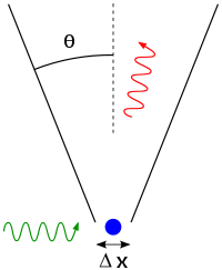
The principle is quite counter-intuitive, so the early students of quantum theory had to be reassured that naive measurements to violate it were bound always to be unworkable. One way in which Heisenberg originally illustrated the intrinsic impossibility of violating the uncertainty principle is by utilizing the observer effect of an imaginary microscope as a measuring device.[69]
He imagines an experimenter trying to measure the position and momentum of an electron by shooting a photon at it.[71]:49–50
- Problem 1 – If the photon has a short wavelength, and therefore, a large momentum, the position can be measured accurately. But the photon scatters in a random direction, transferring a large and uncertain amount of momentum to the electron. If the photon has a long wavelength and low momentum, the collision does not disturb the electron's momentum very much, but the scattering will reveal its position only vaguely.
- Problem 2 – If a large aperture is used for the microscope, the electron's location can be well resolved (see Rayleigh criterion); but by the principle of conservation of momentum, the transverse momentum of the incoming photon affects the electron's beamline momentum and hence, the new momentum of the electron resolves poorly. If a small aperture is used, the accuracy of both resolutions is the other way around.
The combination of these trade-offs implies that no matter what photon wavelength and aperture size are used, the product of the uncertainty in measured position and measured momentum is greater than or equal to a lower limit, which is (up to a small numerical factor) equal to Planck's constant.[72] Heisenberg did not care to formulate the uncertainty principle as an exact limit (which is elaborated below), and preferred to use it instead, as a heuristic quantitative statement, correct up to small numerical factors, which makes the radically new noncommutativity of quantum mechanics inevitable.
Critical reactions
The Copenhagen interpretation of quantum mechanics and Heisenberg's Uncertainty Principle were, in fact, seen as twin targets by detractors who believed in an underlying determinism and realism. According to the Copenhagen interpretation of quantum mechanics, there is no fundamental reality that the quantum state describes, just a prescription for calculating experimental results. There is no way to say what the state of a system fundamentally is, only what the result of observations might be.
Albert Einstein believed that randomness is a reflection of our ignorance of some fundamental property of reality, while Niels Bohr believed that the probability distributions are fundamental and irreducible, and depend on which measurements we choose to perform. Einstein and Bohr debated the uncertainty principle for many years.
The ideal of the detached observer
Wolfgang Pauli called Einstein's fundamental objection to the uncertainty principle "the ideal of the detached observer" (phrase translated from the German):
"Like the moon has a definite position" Einstein said to me last winter, "whether or not we look at the moon, the same must also hold for the atomic objects, as there is no sharp distinction possible between these and macroscopic objects. Observation cannot create an element of reality like a position, there must be something contained in the complete description of physical reality which corresponds to the possibility of observing a position, already before the observation has been actually made." I hope, that I quoted Einstein correctly; it is always difficult to quote somebody out of memory with whom one does not agree. It is precisely this kind of postulate which I call the ideal of the detached observer.
- Letter from Pauli to Niels Bohr, February 15, 1955[73]
Einstein's slit
The first of Einstein's thought experiments challenging the uncertainty principle went as follows:
- Consider a particle passing through a slit of width d. The slit introduces an uncertainty in momentum of approximately h/d because the particle passes through the wall. But let us determine the momentum of the particle by measuring the recoil of the wall. In doing so, we find the momentum of the particle to arbitrary accuracy by conservation of momentum.
Bohr's response was that the wall is quantum mechanical as well, and that to measure the recoil to accuracy Δp, the momentum of the wall must be known to this accuracy before the particle passes through. This introduces an uncertainty in the position of the wall and therefore the position of the slit equal to h/Δp, and if the wall's momentum is known precisely enough to measure the recoil, the slit's position is uncertain enough to disallow a position measurement.
A similar analysis with particles diffracting through multiple slits is given by Richard Feynman.[74]
Einstein's box
Bohr was present when Einstein proposed the thought experiment which has become known as Einstein's box. Einstein argued that "Heisenberg's uncertainty equation implied that the uncertainty in time was related to the uncertainty in energy, the product of the two being related to Planck's constant."[75] Consider, he said, an ideal box, lined with mirrors so that it can contain light indefinitely. The box could be weighed before a clockwork mechanism opened an ideal shutter at a chosen instant to allow one single photon to escape. "We now know, explained Einstein, precisely the time at which the photon left the box."[76] "Now, weigh the box again. The change of mass tells the energy of the emitted light. In this manner, said Einstein, one could measure the energy emitted and the time it was released with any desired precision, in contradiction to the uncertainty principle."[75]
Bohr spent a sleepless night considering this argument, and eventually realized that it was flawed. He pointed out that if the box were to be weighed, say by a spring and a pointer on a scale, "since the box must move vertically with a change in its weight, there will be uncertainty in its vertical velocity and therefore an uncertainty in its height above the table. ... Furthermore, the uncertainty about the elevation above the earth's surface will result in an uncertainty in the rate of the clock,"[77] because of Einstein's own theory of gravity's effect on time. "Through this chain of uncertainties, Bohr showed that Einstein's light box experiment could not simultaneously measure exactly both the energy of the photon and the time of its escape."[78]
EPR paradox for entangled particles
Bohr was compelled to modify his understanding of the uncertainty principle after another thought experiment by Einstein. In 1935, Einstein, Podolsky and Rosen (see EPR paradox) published an analysis of widely separated entangled particles. Measuring one particle, Einstein realized, would alter the probability distribution of the other, yet here the other particle could not possibly be disturbed. This example led Bohr to revise his understanding of the principle, concluding that the uncertainty was not caused by a direct interaction.[79]
But Einstein came to much more far-reaching conclusions from the same thought experiment. He believed the "natural basic assumption" that a complete description of reality would have to predict the results of experiments from "locally changing deterministic quantities" and therefore would have to include more information than the maximum possible allowed by the uncertainty principle.
In 1964, John Bell showed that this assumption can be falsified, since it would imply a certain inequality between the probabilities of different experiments. Experimental results confirm the predictions of quantum mechanics, ruling out Einstein's basic assumption that led him to the suggestion of his hidden variables. These hidden variables may be "hidden" because of an illusion that occurs during observations of objects that are too large or too small. This illusion can be likened to rotating fan blades that seem to pop in and out of existence at different locations and sometimes seem to be in the same place at the same time when observed. This same illusion manifests itself in the observation of subatomic particles. Both the fan blades and the subatomic particles are moving so fast that the illusion is seen by the observer. Therefore, it is possible that there would be predictability of the subatomic particles behavior and characteristics to a recording device capable of very high speed tracking....Ironically this fact is one of the best pieces of evidence supporting Karl Popper's philosophy of invalidation of a theory by falsification-experiments. That is to say, here Einstein's "basic assumption" became falsified by experiments based on Bell's inequalities. For the objections of Karl Popper to the Heisenberg inequality itself, see below.
While it is possible to assume that quantum mechanical predictions are due to nonlocal, hidden variables, and in fact David Bohm invented such a formulation, this resolution is not satisfactory to the vast majority of physicists. The question of whether a random outcome is predetermined by a nonlocal theory can be philosophical, and it can be potentially intractable. If the hidden variables are not constrained, they could just be a list of random digits that are used to produce the measurement outcomes. To make it sensible, the assumption of nonlocal hidden variables is sometimes augmented by a second assumption—that the size of the observable universe puts a limit on the computations that these variables can do. A nonlocal theory of this sort predicts that a quantum computer would encounter fundamental obstacles when attempting to factor numbers of approximately 10,000 digits or more; a potentially achievable task in quantum mechanics.[80]
Popper's criticism
Karl Popper approached the problem of indeterminacy as a logician and metaphysical realist.[81] He disagreed with the application of the uncertainty relations to individual particles rather than to ensembles of identically prepared particles, referring to them as "statistical scatter relations".[81][82] In this statistical interpretation, a particular measurement may be made to arbitrary precision without invalidating the quantum theory. This directly contrasts with the Copenhagen interpretation of quantum mechanics, which is non-deterministic but lacks local hidden variables.
In 1934, Popper published Zur Kritik der Ungenauigkeitsrelationen (Critique of the Uncertainty Relations) in Naturwissenschaften,[83] and in the same year Logik der Forschung (translated and updated by the author as The Logic of Scientific Discovery in 1959), outlining his arguments for the statistical interpretation. In 1982, he further developed his theory in Quantum theory and the schism in Physics, writing:
[Heisenberg's] formulae are, beyond all doubt, derivable statistical formulae of the quantum theory. But they have been habitually misinterpreted by those quantum theorists who said that these formulae can be interpreted as determining some upper limit to the precision of our measurements. [original emphasis][84]
Popper proposed an experiment to falsify the uncertainty relations, although he later withdrew his initial version after discussions with Weizsäcker, Heisenberg, and Einstein; this experiment may have influenced the formulation of the EPR experiment.[81][85]
Many-worlds uncertainty
The many-worlds interpretation originally outlined by Hugh Everett III in 1957 is partly meant to reconcile the differences between Einstein's and Bohr's views by replacing Bohr's wave function collapse with an ensemble of deterministic and independent universes whose distribution is governed by wave functions and the Schrödinger equation. Thus, uncertainty in the many-worlds interpretation follows from each observer within any universe having no knowledge of what goes on in the other universes.
Free will
Some scientists including Arthur Compton[86] and Martin Heisenberg[87] have suggested that the uncertainty principle, or at least the general probabilistic nature of quantum mechanics, could be evidence for the two-stage model of free will. One critique, however, is that apart from the basic role of quantum mechanics as a foundation for chemistry, nontrivial biological mechanisms requiring quantum mechanics are unlikely, due to the rapid decoherence time of quantum systems at room temperature.[88] The standard view, however, is that this decoherence is overcome by both screening and decoherence-free subspaces found in biological cells.[88]
The second law of thermodynamics
There is reason to believe that violating the uncertainty principle also strongly implies the violation of the second law of thermodynamics.[89]
See also
- Afshar experiment
- Canonical commutation relation
- Correspondence principle
- Correspondence rules
- Gromov's non-squeezing theorem
- Discrete Fourier transform#Uncertainty principle
- Einstein's thought experiments
- Heisenbug
- Introduction to quantum mechanics
- Operationalization
- Observer effect (information technology)
- Observer effect (physics)
- Quantum indeterminacy
- Quantum non-equilibrium
- Quantum tunnelling
- Physics and Beyond (book)
- Stronger uncertainty relations
- Weak measurement
Notes
- ↑ N.B. on precision: If and are the precisions of position and momentum obtained in an individual measurement and , their standard deviations in an ensemble of individual measurements on similarly prepared systems, then "There are, in principle, no restrictions on the precisions of individual measurements and , but the standard deviations will always satisfy ".[11]


References
- 1 2 3 Sen, D. (2014). "The Uncertainty relations in quantum mechanics" (PDF). Current Science. 107 (2): 203–218.
- 1 2 3 Heisenberg, W. (1927), "Über den anschaulichen Inhalt der quantentheoretischen Kinematik und Mechanik", Zeitschrift für Physik (in German), 43 (3–4): 172–198, Bibcode:1927ZPhy...43..172H, doi:10.1007/BF01397280. . Annotated pre-publication proof sheet of Über den anschaulichen Inhalt der quantentheoretischen Kinematik und Mechanik, March 21, 1927.
- 1 2 3 Kennard, E. H. (1927), "Zur Quantenmechanik einfacher Bewegungstypen", Zeitschrift für Physik (in German), 44 (4–5): 326–352, Bibcode:1927ZPhy...44..326K, doi:10.1007/BF01391200.
- ↑ Weyl, H. (1928), Gruppentheorie und Quantenmechanik, Leipzig: Hirzel
- ↑ Furuta, Aya (2012), "One Thing Is Certain: Heisenberg's Uncertainty Principle Is Not Dead", Scientific American
- 1 2 Ozawa, Masanao (2003), "Universally valid reformulation of the Heisenberg uncertainty principle on noise and disturbance in measurement", Physical Review A, 67 (4): 42105, arXiv:quant-ph/0207121, Bibcode:2003PhRvA..67d2105O, doi:10.1103/PhysRevA.67.042105
- ↑ Werner Heisenberg, The Physical Principles of the Quantum Theory, p. 20
- 1 2 Rozema, L. A.; Darabi, A.; Mahler, D. H.; Hayat, A.; Soudagar, Y.; Steinberg, A. M. (2012). "Violation of Heisenberg's Measurement–Disturbance Relationship by Weak Measurements". Physical Review Letters. 109 (10): 100404. arXiv:1208.0034v2. Bibcode:2012PhRvL.109j0404R. doi:10.1103/PhysRevLett.109.100404. PMID 23005268.
- ↑ Indian Institute of Technology Madras, Professor V. Balakrishnan, Lecture 1 – Introduction to Quantum Physics; Heisenberg's uncertainty principle, National Programme of Technology Enhanced Learning on YouTube
- 1 2 3 4 L.D. Landau, E. M. Lifshitz (1977). Quantum Mechanics: Non-Relativistic Theory. Vol. 3 (3rd ed.). Pergamon Press. ISBN 978-0-08-020940-1. Online copy.
- ↑ Section 3.2 of Ballentine, Leslie E. (1970), "The Statistical Interpretation of Quantum Mechanics", Reviews of Modern Physics, 42 (4): 358–381, Bibcode:1970RvMP...42..358B, doi:10.1103/RevModPhys.42.358 . This fact is experimentally well-known for example in quantum optics (see e.g. chap. 2 and Fig. 2.1 Leonhardt, Ulf (1997), Measuring the Quantum State of Light, Cambridge: Cambridge University Press, ISBN 0 521 49730 2
- ↑ Elion, W. J.; M. Matters, U. Geigenmüller & J. E. Mooij; Geigenmüller, U.; Mooij, J. E. (1994), "Direct demonstration of Heisenberg's uncertainty principle in a superconductor", Nature, 371 (6498): 594–595, Bibcode:1994Natur.371..594E, doi:10.1038/371594a0
- ↑ Smithey, D. T.; M. Beck, J. Cooper, M. G. Raymer; Cooper, J.; Raymer, M. G. (1993), "Measurement of number–phase uncertainty relations of optical fields", Phys. Rev. A, 48 (4): 3159–3167, Bibcode:1993PhRvA..48.3159S, doi:10.1103/PhysRevA.48.3159, PMID 9909968
- ↑ Caves, Carlton (1981), "Quantum-mechanical noise in an interferometer", Phys. Rev. D, 23 (8): 1693–1708, Bibcode:1981PhRvD..23.1693C, doi:10.1103/PhysRevD.23.1693
- ↑ Jaeger, Gregg (September 2014). "What in the (quantum) world is macroscopic?". American Journal of Physics. 82 (9): 896–905. Bibcode:2014AmJPh..82..896J. doi:10.1119/1.4878358.
- ↑ Claude Cohen-Tannoudji; Bernard Diu; Franck Laloë (1996), Quantum mechanics, Wiley-Interscience: Wiley, pp. 231–233, ISBN 978-0-471-56952-7
- 1 2 Robertson, H. P. (1929), "The Uncertainty Principle", Phys. Rev., 34: 163–64, Bibcode:1929PhRv...34..163R, doi:10.1103/PhysRev.34.163
- 1 2 Schrödinger, E. (1930), "Zum Heisenbergschen Unschärfeprinzip", Sitzungsberichte der Preussischen Akademie der Wissenschaften, Physikalisch-mathematische Klasse, 14: 296–303
- 1 2 Griffiths, David (2005), Quantum Mechanics, New Jersey: Pearson
- ↑ Riley, K. F.; M. P. Hobson and S. J. Bence (2006), Mathematical Methods for Physics and Engineering, Cambridge, p. 246
- ↑ Davidson, E. R. (1965), "On Derivations of the Uncertainty Principle", J. Chem. Phys., 42 (4): 1461, Bibcode:1965JChPh..42.1461D, doi:10.1063/1.1696139
- 1 2 3 Hall, B. C. (2013), Quantum Theory for Mathematicians, Springer, p. 245
- ↑ Jackiw, Roman (1968), "Minimum Uncertainty Product, Number‐Phase Uncertainty Product, and Coherent States", J. Math. Phys., 9 (3): 339, Bibcode:1968JMP.....9..339J, doi:10.1063/1.1664585
- 1 2 Carruthers, P.; Nieto, M. M. (1968), "Phase and Angle Variables in Quantum Mechanics", Rev. Mod. Phys., 40 (2): 411–440, Bibcode:1968RvMP...40..411C, doi:10.1103/RevModPhys.40.411
- ↑ Hall, B. C. (2013), Quantum Theory for Mathematicians, Springer
- ↑ L. I. Mandelshtam, I. E. Tamm, The uncertainty relation between energy and time in nonrelativistic quantum mechanics, 1945.
- ↑ Hilgevoord, Jan (1996). "The uncertainty principle for energy and time" (PDF). American Journal of Physics. 64 (12): 1451–1456. Bibcode:1996AmJPh..64.1451H. doi:10.1119/1.18410. ; Hilgevoord, Jan (1998). "The uncertainty principle for energy and time. II". American Journal of Physics. 66 (5): 396–402. Bibcode:1998AmJPh..66..396H. doi:10.1119/1.18880.
- ↑ The broad linewidth of fast-decaying states makes it difficult to accurately measure the energy of the state, and researchers have even used detuned microwave cavities to slow down the decay rate, to get sharper peaks. Gabrielse, Gerald; H. Dehmelt (1985), "Observation of Inhibited Spontaneous Emission", Physical Review Letters, 55 (1): 67–70, Bibcode:1985PhRvL..55...67G, doi:10.1103/PhysRevLett.55.67, PMID 10031682
- ↑ Likharev, K. K.; A. B. Zorin (1985), "Theory of Bloch-Wave Oscillations in Small Josephson Junctions", J. Low Temp. Phys., 59 (3/4): 347–382, Bibcode:1985JLTP...59..347L, doi:10.1007/BF00683782
- ↑ Anderson, P. W. (1964), "Special Effects in Superconductivity", in Caianiello, E. R., Lectures on the Many-Body Problem, Vol. 2, New York: Academic Press
- ↑ More precisely, whenever both and are defined, and the space of such is a dense subspace of the quantum Hilbert space. See Hall, B. C. (2013), Quantum Theory for Mathematicians, Springer, p. 245
- ↑ Hall, B. C. (2013), Quantum Theory for Mathematicians, Springer, p. 285
- ↑ Hall, B. C. (2013), Quantum Theory for Mathematicians, Springer, p. 246
- ↑ Steiger, Nathan. "Quantum Uncertainty and Conservation Law Restrictions on Gate Fidelity". Brigham Young University. Retrieved 19 June 2011.
- ↑ Maccone, Lorenzo; Pati, Arun K. (31 December 2014). "Stronger Uncertainty Relations for All Incompatible Observables". Physical Review Letters. 113 (26): 260401. arXiv:1407.0338. Bibcode:2014PhRvL.113z0401M. doi:10.1103/PhysRevLett.113.260401.
- ↑ Curtright, T.; Zachos, C. (2001). "Negative Probability and Uncertainty Relations". Modern Physics Letters A. 16 (37): 2381–2385. arXiv:hep-th/0105226. Bibcode:2001MPLA...16.2381C. doi:10.1142/S021773230100576X.
- ↑ Busch, P.; Lahti, P.; Werner, R. F. (2013). "Proof of Heisenberg's Error-Disturbance Relation". Physical Review Letters. 111 (16): 160405. arXiv:1306.1565. Bibcode:2013PhRvL.111p0405B. doi:10.1103/PhysRevLett.111.160405. PMID 24182239.
- ↑ Busch, P.; Lahti, P.; Werner, R. F. (2014). "Heisenberg uncertainty for qubit measurements". Physical Review A. 89. arXiv:1311.0837. Bibcode:2014PhRvA..89a2129B. doi:10.1103/PhysRevA.89.012129.
- ↑ Erhart, J.; Sponar, S.; Sulyok, G.; Badurek, G.; Ozawa, M.; Hasegawa, Y. (2012). "Experimental demonstration of a universally valid error-disturbance uncertainty relation in spin measurements". Nature Physics. 8 (3): 185–189. arXiv:1201.1833. Bibcode:2012NatPh...8..185E. doi:10.1038/nphys2194.
- ↑ Baek, S.-Y.; Kaneda, F.; Ozawa, M.; Edamatsu, K. (2013). "Experimental violation and reformulation of the Heisenberg's error-disturbance uncertainty relation". Scientific Reports. 3: 2221. Bibcode:2013NatSR...3E2221B. doi:10.1038/srep02221. PMC 3713528. PMID 23860715.
- ↑ Ringbauer, M.; Biggerstaff, D.N.; Broome, M.A.; Fedrizzi, A.; Branciard, C.; White, A.G. (2014). "Experimental Joint Quantum Measurements with Minimum Uncertainty". Physical Review Letters. 112: 020401. arXiv:1308.5688. Bibcode:2014PhRvL.112b0401R. doi:10.1103/PhysRevLett.112.020401. PMID 24483993.
- ↑ Björk, G.; Söderholm, J.; Trifonov, A.; Tsegaye, T.; Karlsson, A. (1999). "Complementarity and the uncertainty relations". Physical Review. A60: 1878. arXiv:quant-ph/9904069. Bibcode:1999PhRvA..60.1874B. doi:10.1103/PhysRevA.60.1874.
- ↑ Fujikawa, Kazuo (2012). "Universally valid Heisenberg uncertainty relation". Physical Review A. 85 (6). arXiv:1205.1360. Bibcode:2012PhRvA..85f2117F. doi:10.1103/PhysRevA.85.062117.
- ↑ Judge, D. (1964), "On the uncertainty relation for angle variables", Il Nuovo Cimento, 31 (2): 332–340, Bibcode:1964NCim...31..332J, doi:10.1007/BF02733639
- ↑ Bouten, M.; Maene, N.; Van Leuven, P. (1965), "On an uncertainty relation for angle variables", Il Nuovo Cimento, 37 (3): 1119–1125, Bibcode:1965NCim...37.1119B, doi:10.1007/BF02773197
- ↑ Louisell, W. H. (1963), "Amplitude and phase uncertainty relations", Physics Letters, 7 (1): 60–61, Bibcode:1963PhL.....7...60L, doi:10.1016/0031-9163(63)90442-6
- ↑ DeWitt, B. S.; Graham, N. (1973), The Many-Worlds Interpretation of Quantum Mechanics, Princeton: Princeton University Press, pp. 52–53, ISBN 0-691-08126-3
- ↑ Hirschman, I. I., Jr. (1957), "A note on entropy", American Journal of Mathematics, 79 (1): 152–156, doi:10.2307/2372390, JSTOR 2372390.
- ↑ Beckner, W. (1975), "Inequalities in Fourier analysis", Annals of Mathematics, 102 (6): 159–182, doi:10.2307/1970980, JSTOR 1970980.
- ↑ Bialynicki-Birula, I.; Mycielski, J. (1975), "Uncertainty Relations for Information Entropy in Wave Mechanics", Communications in Mathematical Physics, 44 (2): 129–132, Bibcode:1975CMaPh..44..129B, doi:10.1007/BF01608825
- ↑ Chafaï, D. (2003), Gaussian maximum of entropy and reversed log-Sobolev inequality, pp. 194–200, arXiv:math/0102227, doi:10.1007/978-3-540-36107-7_5, ISBN 978-3-540-00072-3
- ↑ Havin, V.; Jöricke, B. (1994), The Uncertainty Principle in Harmonic Analysis, Springer-Verlag
- ↑ Folland, Gerald; Sitaram, Alladi (May 1997), "The Uncertainty Principle: A Mathematical Survey", Journal of Fourier Analysis and Applications, 3 (3): 207–238, doi:10.1007/BF02649110, MR 1448337
- ↑ Sitaram, A (2001) [1994], "Uncertainty principle, mathematical", in Hazewinkel, Michiel, Encyclopedia of Mathematics, Springer Science+Business Media B.V. / Kluwer Academic Publishers, ISBN 978-1-55608-010-4
- ↑ Matt Hall, "What is the Gabor uncertainty principle?"
- ↑ Donoho, D.L.; Stark, P.B (1989). "Uncertainty principles and signal recovery". SIAM Journal on Applied Mathematics. 49 (3): 906–931. doi:10.1137/0149053.
- ↑ Amrein, W.O.; Berthier, A.M. (1977), "On support properties of Lp-functions and their Fourier transforms", Journal of Functional Analysis, 24 (3): 258–267, doi:10.1016/0022-1236(77)90056-8.
- ↑ Benedicks, M. (1985), "On Fourier transforms of functions supported on sets of finite Lebesgue measure", J. Math. Anal. Appl., 106 (1): 180–183, doi:10.1016/0022-247X(85)90140-4
- ↑ Nazarov, F. (1994), "Local estimates for exponential polynomials and their applications to inequalities of the uncertainty principle type", St. Petersburg Math. J., 5: 663–717
- ↑ Jaming, Ph. (2007), "Nazarov's uncertainty principles in higher dimension", J. Approx. Theory, 149 (1): 30–41, doi:10.1016/j.jat.2007.04.005
- ↑ Hardy, G.H. (1933), "A theorem concerning Fourier transforms", Journal of the London Mathematical Society, 8 (3): 227–231, doi:10.1112/jlms/s1-8.3.227
- ↑ Hörmander, L. (1991), "A uniqueness theorem of Beurling for Fourier transform pairs", Ark. Mat., 29: 231–240, Bibcode:1991ArM....29..237H, doi:10.1007/BF02384339
- ↑ Bonami, A.; Demange, B.; Jaming, Ph. (2003), "Hermite functions and uncertainty principles for the Fourier and the windowed Fourier transforms", Rev. Mat. Iberoamericana, 19: 23–55., arXiv:math/0102111, Bibcode:2001math......2111B, doi:10.4171/RMI/337
- ↑ Hedenmalm, H. (2012), "Heisenberg's uncertainty principle in the sense of Beurling", J. Anal. Math., 118 (2): 691–702, arXiv:1203.5222, doi:10.1007/s11854-012-0048-9
- ↑ Demange, Bruno (2009), Uncertainty Principles Associated to Non-degenerate Quadratic Forms, Société Mathématique de France, ISBN 978-2-85629-297-6
- ↑ American Physical Society online exhibit on the Uncertainty Principle
- ↑ Bohr, Niels; Noll, Waldemar (1958), "Atomic Physics and Human Knowledge", American Journal of Physics, New York: Wiley, 26 (8): 38, Bibcode:1958AmJPh..26..596B, doi:10.1119/1.1934707
- ↑ Heisenberg, W., Die Physik der Atomkerne, Taylor & Francis, 1952, p. 30.
- 1 2 3 Heisenberg, W. (1930), Physikalische Prinzipien der Quantentheorie (in German), Leipzig: Hirzel English translation The Physical Principles of Quantum Theory. Chicago: University of Chicago Press, 1930.
- ↑ Cassidy, David; Saperstein, Alvin M. (2009), "Beyond Uncertainty: Heisenberg, Quantum Physics, and the Bomb", Physics Today, New York: Bellevue Literary Press, 63: 185, Bibcode:2010PhT....63a..49C, doi:10.1063/1.3293416
- ↑ George Greenstein; Arthur Zajonc (2006). The Quantum Challenge: Modern Research on the Foundations of Quantum Mechanics. Jones & Bartlett Learning. ISBN 978-0-7637-2470-2.
- ↑ Tipler, Paul A.; Llewellyn, Ralph A. (1999), "5–5", Modern Physics (3rd ed.), W. H. Freeman and Co., ISBN 1-57259-164-1
- ↑ Enz, Charles P.; Meyenn, Karl von, eds. (1994). Writings on physics and philosophy by Wolfgang Pauli. Springer-Verlag. p. 43. ISBN 3-540-56859-X; translated by Robert Schlapp
- ↑ Feynman lectures on Physics, vol 3, 2–2
- 1 2 Gamow, G., The great physicists from Galileo to Einstein, Courier Dover, 1988, p.260.
- ↑ Kumar, M., Quantum: Einstein, Bohr and the Great Debate About the Nature of Reality, Icon, 2009, p. 282.
- ↑ Gamow, G., The great physicists from Galileo to Einstein, Courier Dover, 1988, p. 260–261.
- ↑ Kumar, M., Quantum: Einstein, Bohr and the Great Debate About the Nature of Reality, Icon, 2009, p. 287.
- ↑ Isaacson, Walter (2007), Einstein: His Life and Universe, New York: Simon & Schuster, p. 452, ISBN 978-0-7432-6473-0
- ↑ Gerardus 't Hooft has at times advocated this point of view.
- 1 2 3 Popper, Karl (1959), The Logic of Scientific Discovery, Hutchinson & Co.
- ↑ Jarvie, Ian Charles; Milford, Karl; Miller, David W (2006), Karl Popper: a centenary assessment, 3, Ashgate Publishing, ISBN 978-0-7546-5712-5
- ↑ Popper, Karl; Carl Friedrich von Weizsäcker (1934), "Zur Kritik der Ungenauigkeitsrelationen (Critique of the Uncertainty Relations)", Naturwissenschaften, 22 (48): 807–808, Bibcode:1934NW.....22..807P, doi:10.1007/BF01496543.
- ↑ Popper, K. Quantum theory and the schism in Physics, Unwin Hyman Ltd, 1982, pp. 53–54.
- ↑ Mehra, Jagdish; Rechenberg, Helmut (2001), The Historical Development of Quantum Theory, Springer, ISBN 978-0-387-95086-0
- ↑ Compton, A. H. (1931). "The Uncertainty Principle and Free Will". Science. 74 (1911): 172. Bibcode:1931Sci....74..172C. doi:10.1126/science.74.1911.172. PMID 17808216.
- ↑ Heisenberg, M. (2009). "Is free will an illusion?". Nature. 459 (7244): 164–165. Bibcode:2009Natur.459..164H. doi:10.1038/459164a.
- 1 2 Davies, P. C. W. (2004). "Does quantum mechanics play a non-trivial role in life?". Biosystems. 78 (1–3): 69–79. doi:10.1016/j.biosystems.2004.07.001. PMID 15555759.
- ↑ E. Hanggi, S. Wehner, A violation of the uncertainty principle also implies the violation of the second law of thermodynamics; 2012, arXiv:1205.6894v1 (quant-phy).

External links
| Wikiquote has quotations related to: Uncertainty principle |
- Hazewinkel, Michiel, ed. (2001) [1994], "Uncertainty principle", Encyclopedia of Mathematics, Springer Science+Business Media B.V. / Kluwer Academic Publishers, ISBN 978-1-55608-010-4
- Matter as a Wave – a chapter from an online textbook
- Quantum mechanics: Myths and facts
- Stanford Encyclopedia of Philosophy entry
- Fourier Transforms and Uncertainty at MathPages
- aip.org: Quantum mechanics 1925–1927 – The uncertainty principle
- Eric Weisstein's World of Physics – Uncertainty principle
- John Baez on the time–energy uncertainty relation
- The certainty principle
- Common Interpretation of Heisenberg's Uncertainty Principle Is Proved False