Basis (linear algebra)

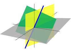
The same vector can be represented in two different bases (purple and red arrows).

In mathematics, a set of elements (vectors) in a vector space V is called a basis, or a set of basis vectors, if the vectors are linearly independent and every vector in the vector space is a linear combination of this set.^[1] In more general terms, a basis is a linearly independent spanning set.

Given a basis of a vector space V, every element of V can be expressed uniquely as a linear combination of basis vectors, whose coefficients are referred to as vector coordinates or components. The computation of these components is sometimes called decomposition of a vector on a basis. A vector space can have several distinct sets of basis vectors; however each such set has the same number of elements, with this number being the dimension of the vector space.

Definition

This picture illustrates the standard basis in R². The blue and orange vectors are the elements of the basis; the green vector can be given in terms of the basis vectors, and so is linearly dependent upon them.

A basis B of a vector space V over a field F is a linearly independent subset of V that spans V.

In more detail, suppose that B = { v₁, …, v_n } is a finite subset of a vector space V over a field F (such as the real or complex numbers R or C). Then B is a basis if it satisfies the following conditions:

the linear independence property,

for all a₁, …, a_n ∈ F, if a₁v₁ + … + a_nv_n = 0, then necessarily a₁ = … = a_n = 0; and

the spanning property,

for every (vector) x in V it is possible to choose a₁, …, a_n ∈ F such that x = a₁v₁ + … + a_nv_n.

The numbers a_i are called the coordinates of the vector x with respect to the basis B, and by the first property they are uniquely determined.

A vector space that has a finite basis is called finite-dimensional. To deal with infinite-dimensional spaces, we must generalize the above definition to include infinite basis sets. We therefore say that a set (finite or infinite) B ⊂ V is a basis, if

every finite subset B₀ ⊆ B obeys the independence property shown above; and
for every x in V it is possible to choose a₁, …, a_n ∈ F and v₁, …, v_n ∈ B such that x = a₁v₁ + … + a_nv_n.

The sums in the above definition are all finite because without additional structure the axioms of a vector space do not permit us to meaningfully speak about an infinite sum of vectors. Settings that permit infinite linear combinations allow alternative definitions of the basis concept: see Related notions below.

It is often convenient to list the basis vectors in a specific order, for example, when considering the transformation matrix of a linear map with respect to a basis. We then speak of an ordered basis, which we define to be a sequence (rather than a set) of linearly independent vectors that span V: see Ordered bases and coordinates below.

Properties

Again, B denotes a subset of a vector space V. Then, B is a basis if and only if any of the following equivalent conditions are met:

B is a minimal generating set of V, i.e., it is a generating set and no proper subset of B is also a generating set.
B is a maximal set of linearly independent vectors, i.e., it is a linearly independent set but no other linearly independent set contains it as a proper subset.
Every vector in V can be expressed as a linear combination of vectors in B in a unique way. If the basis is ordered (see Ordered bases and coordinates below) then the coefficients in this linear combination provide coordinates of the vector relative to the basis.

Every vector space has a basis. The proof of this requires the axiom of choice. All bases of a vector space have the same cardinality (number of elements), called the dimension of the vector space. This result is known as the dimension theorem, and requires the ultrafilter lemma, a strictly weaker form of the axiom of choice.

Also many vector sets can be attributed a standard basis which comprises both spanning and linearly independent vectors.

Standard bases for example:

In Rⁿ, {e₁, ..., e_n}, where e_i is the ith column of the identity matrix.

In P₂, where P₂ is the set of all polynomials of degree at most 2, {1, x, x²} is the standard basis.

In M₂₂, {M_1,1, M_1,2, M_2,1, M_2,2}, where M₂₂ is the set of all 2×2 matrices and M_m,n is the 2×2 matrix with a 1 in the m,n position and zeros everywhere else.

Change of basis

Given a vector space V over a field F and suppose that {v₁, ..., v_n} and {α₁, ..., α_n} are two bases for V. By definition, if ξ is a vector in V then ξ = x₁α₁ + ... + x_nα_n for a unique choice of scalars x₁, ..., x_n in F called the coordinates of ξ relative to the ordered basis {α₁, ..., α_n}. The vector x = (x₁, ..., x_n) in Fⁿ is called the coordinate tuple of ξ (relative to this basis). The unique linear map φ : Fⁿ → V with φ(v_j) = α_j for j = 1, ..., n is called the coordinate isomorphism for V and the basis {α₁, ..., α_n}. Thus φ(x) = ξ if and only if ξ = x₁α₁ + ... + x_nα_n.

A set of vectors can be represented by a matrix of which each column consists of the components of the corresponding vector of the set. As a basis is a set of vectors, a basis can be given by a matrix of this kind. The change of basis of any object of the space is related to this matrix. For example, coordinate tuples change with its inverse.

Examples

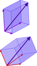
Consider R², the vector space of all coordinates (a, b) where both a and b are real numbers. Then a very natural and simple basis is simply the vectors e₁ = (1,0) and e₂ = (0,1): suppose that v = (a, b) is a vector in R², then v = a(1,0) + b(0,1). But any two linearly independent vectors, like (1,1) and (−1,2), will also form a basis of R².
More generally, the vectors e₁, e₂, ..., e_n are linearly independent and generate Rⁿ. Therefore, they form a basis for Rⁿ and the dimension of Rⁿ is n. This basis is called the standard basis.
Let V be the real vector space generated by the functions e^t and e^2t. These two functions are linearly independent, so they form a basis for V.
Let R[x] denote the vector space of real polynomials; then (1, x, x², ...) is a basis of R[x]. The dimension of R[x] is therefore equal to aleph-0.

Extending to a basis

Let S be a subset of a vector space V. To extend S to a basis of V means to find a basis B of V that contains S as a subset. This can be done if and only if S is linearly independent. Almost always, there is more than one such B, except in rather special circumstances (i.e. that S is already a basis, or S is empty and V has two elements).

A similar question is when does a subset S contain a basis. This occurs if and only if S spans V. In this case, S will usually contain several different bases.

Example of alternative proofs

Often, a mathematical result can be proven in more than one way. Here, using three different proofs, we show that the vectors (1,1) and (−1,2) form a basis for R².

From the definition of basis

We have to prove that these two vectors are linearly independent and that they generate R².

Part I: If two vectors v and w are linearly independent, then $av+bw=0$ (a and b scalars) implies $a=0,b=0$ .

To prove that they are linearly independent, suppose that there are numbers a, b such that:

a(1,1)+b(-1,2)=(0,0)

(i.e., they are linearly dependent). Then:

(a-b,a+2b)=(0,0)

and

a-b=0

and

a+2b=0.

Subtracting the first equation from the second, we obtain:

3b=0

so

b=0.

Adding this equation to the first equation then:

a=0.

Hence we have linear independence.

Part II: To prove that these two vectors generate R², we have to let (a, b) be an arbitrary element of R², and show that there exist numbers r, s ∈ R such that:

r(1,1)+s(-1,2)=(a,b).

Then we have to solve the equations:

r-s=a

r+2s=b.

Subtracting the first equation from the second, we get:

3s=b-a,

and then

s=(b-a)/3,

and finally

r=s+a=((b-a)/3)+a=(b+2a)/3.

By the dimension theorem

Since (−1,2) is clearly not a multiple of (1,1) and since (1,1) is not the zero vector, these two vectors are linearly independent. Since the dimension of R² is 2, the two vectors already form a basis of R² without needing any extension.

By the invertible matrix theorem

Simply compute the determinant

\det {\begin{bmatrix}1&-1\\1&2\end{bmatrix}}=3\neq 0.

Since the above matrix has a nonzero determinant, its columns form a basis of R². See: invertible matrix.

Ordered bases and coordinates

A basis is a linearly independent set of vectors with or without a given ordering. For many purposes it is convenient to work with an ordered basis. For example, when working with a coordinate representation of a vector it is customary to speak of the "first" or "second" coordinate, which makes sense only if an ordering is specified for the basis. For finite-dimensional vector spaces one typically indexes a basis {v_i} by the first n integers. An ordered basis is also called a frame.

Suppose V is an n-dimensional vector space over a field F. A choice of an ordered basis for V is equivalent to a choice of a linear isomorphism φ from the coordinate space Fⁿ to V.

Proof. The proof makes use of the fact that the standard basis of Fⁿ is an ordered basis.

Suppose first that

φ : Fⁿ → V

is a linear isomorphism. Define an ordered basis {v_i} for V by

v_i = φ(e_i) for 1 ≤ i ≤ n

where {e_i} is the standard basis for Fⁿ.

Conversely, given an ordered basis, consider the map defined by

φ(x) = x₁v₁ + x₂v₂ + ... + x_nv_n,

where x = x₁e₁ + x₂e₂ + ... + x_ne_n is an element of Fⁿ. It is not hard to check that φ is a linear isomorphism.

These two constructions are clearly inverse to each other. Thus ordered bases for V are in 1-1 correspondence with linear isomorphisms Fⁿ → V.

The inverse of the linear isomorphism φ determined by an ordered basis {v_i} equips V with coordinates: if, for a vector v ∈ V, φ⁻¹(v) = (a₁, a₂,...,a_n) ∈ Fⁿ, then the components a_j = a_j(v) are the coordinates of v in the sense that v = a₁(v) v₁ + a₂(v) v₂ + ... + a_n(v) v_n.

The maps sending a vector v to the components a_j(v) are linear maps from V to F, because of φ⁻¹ is linear. Hence they are linear functionals. They form a basis for the dual space of V, called the dual basis.

Related notions

Analysis

In the context of infinite-dimensional vector spaces over the real or complex numbers, the term Hamel basis (named after Georg Hamel) or algebraic basis can be used to refer to a basis as defined in this article. This is to make a distinction with other notions of "basis" that exist when infinite-dimensional vector spaces are endowed with extra structure. The most important alternatives are orthogonal bases on Hilbert spaces, Schauder bases, and Markushevich bases on normed linear spaces. In the case of the real numbers R viewed as a vector space over the field Q of rational numbers, Hamel bases are uncountable, and have specifically the cardinality of the continuum, which is the cardinal number $2^{\aleph _{0}},$ where $\aleph _{0}$ is the smallest infinite cardinal, the cardinal of the integers.

The common feature of the other notions is that they permit the taking of infinite linear combinations of the basis vectors in order to generate the space. This, of course, requires that infinite sums are meaningfully defined on these spaces, as is the case for topological vector spaces – a large class of vector spaces including e.g. Hilbert spaces, Banach spaces, or Fréchet spaces.

The preference of other types of bases for infinite-dimensional spaces is justified by the fact that the Hamel basis becomes "too big" in Banach spaces: If X is an infinite-dimensional normed vector space which is complete (i.e. X is a Banach space), then any Hamel basis of X is necessarily uncountable. This is a consequence of the Baire category theorem. The completeness as well as infinite dimension are crucial assumptions in the previous claim. Indeed, finite-dimensional spaces have by definition finite bases and there are infinite-dimensional (non-complete) normed spaces which have countable Hamel bases. Consider $c_{00}$ , the space of the sequences $x=(x_{n})$ of real numbers which have only finitely many non-zero elements, with the norm $\|x\|=\sup _{n}|x_{n}|.$ Its standard basis, consisting of the sequences having only one non-zero element, which is equal to 1, is a countable Hamel basis.

Example

In the study of Fourier series, one learns that the functions {1} ∪ { sin(nx), cos(nx) : n = 1, 2, 3, ... } are an "orthogonal basis" of the (real or complex) vector space of all (real or complex valued) functions on the interval [0, 2π] that are square-integrable on this interval, i.e., functions f satisfying

\int _{0}^{2\pi }\left|f(x)\right|^{2}\,dx<\infty .

The functions {1} ∪ { sin(nx), cos(nx) : n = 1, 2, 3, ... } are linearly independent, and every function f that is square-integrable on [0, 2π] is an "infinite linear combination" of them, in the sense that

\lim _{n\rightarrow \infty }\int _{0}^{2\pi }{\biggl |}a_{0}+\sum _{k=1}^{n}{\bigl (}a_{k}\cos(kx)+b_{k}\sin(kx){\bigr )}-f(x){\biggr |}^{2}\,dx=0

for suitable (real or complex) coefficients a_k, b_k. But many^[2] square-integrable functions cannot be represented as finite linear combinations of these basis functions, which therefore do not comprise a Hamel basis. Every Hamel basis of this space is much bigger than this merely countably infinite set of functions. Hamel bases of spaces of this kind are typically not useful, whereas orthonormal bases of these spaces are essential in Fourier analysis.

Geometry

The geometric notions of an affine space, projective space, convex set, and cone have related notions of basis.^[3] An affine basis for an n-dimensional affine space is $n+1$ points in general linear position. A projective basis is $n+2$ points in general position, in a projective space of dimension n. A convex basis of a polytope is the set of the vertices of its convex hull. A cone basis^[4] consists of one point by edge of a polygonal cone. See also a Hilbert basis (linear programming).

Random basis

For a probability distribution in Rⁿ with a probability density function, such as the equidistribution in a n-dimensional ball with respect to Lebesgue measure, it can be shown that n randomly and independently chosen vectors will form a basis with probability one, which is due to the fact that n linearly dependent vectors x₁, ..., x_n in Rⁿ should satisfy the equation det[x₁, ..., x_n] = 0 (zero determinant of the matrix with columns x_i), and the set of zeros of a non-trivial polynomial has zero measure. This observation has led to techniques for approximating random bases.^[5]^[6]

Empirical distribution of lengths N of pairwise almost orthogonal chains of vectors that are independently randomly sampled from the n-dimensional cube [−1, 1]ⁿ as a function of dimension, n. Boxplots show the second and third quartiles of this data for each n, red bars correspond to the medians, and blue stars indicate means. Red curve shows theoretical bound given by Eq. (1) and green curve shows a refined estimate.^[6]

It is difficult to check numerically the linear dependence or exact orthogonality. Therefore, the notion of ε-orthogonality is used. For spaces with inner product, x is ε-orthogonal to y if $|\langle x,y\rangle |/(\|x\|\|y\|)<\epsilon$ (that is, cosine of the angle between x and y is less than ε).

In high dimensions, two independent random vectors are with high probability almost orthogonal, and the number of independent random vectors, which all are with given high probability pairwise almost orthogonal, grows exponentially with dimension. More precisely, consider equidistribution in n-dimensional ball. Choose N independent random vectors from a ball (they are independent and identically distributed). Let θ be a small positive number. Then for

$N\leq e^{\frac {\epsilon ^{2}n}{4}}[-\ln(1-\theta )]^{\frac {1}{2}}$

(Eq. 1)

N random vectors are all pairwise ε-orthogonal with probability 1 − θ.^[6] This N growth exponentially with dimension n and $N\gg n$ for sufficiently big n. This property of random bases is a manifestation of the so-called measure concentration phenomenon.^[7]

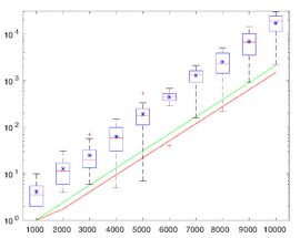
The figure (right) illustrates distribution of lengths N of pairwise almost orthogonal chains of vectors that are independently randomly sampled from the n-dimensional cube [−1, 1]ⁿ as a function of dimension, n. A point is first randomly selected in the cube. The second point is randomly chosen in the same cube. If the angle between the vectors was within π/2 ± 0.037π/2 then the vector was retained. At the next step a new vector is generated in the same hypercube, and its angles with the previously generated vectors are evaluated. If these angles are within π/2 ± 0.037π/2 then the vector is retained. The process is repeated until the chain of almost orthogonality breaks, and the number of such pairwise almost orthogonal vectors (length of the chain) is recorded. For each n, 20 pairwise almost orthogonal chains where constructed numerically for each dimension. Distribution of the length of these chains is presented.

Proof that every vector space has a basis

Let V be any vector space over some field F. Let X be the set of all linearly independent subsets of V.

The set X is nonempty since the empty set is an independent subset of V, and it is partially ordered by inclusion, which is denoted, as usual, by $\subseteq$ .

Let Y be a subset of X that is totally ordered by $\subseteq$ , and let L_Y be the union of all the elements of Y (which are themselves certain subsets of V).

Since (Y, ⊆) is totally ordered, every finite subset of L_Y is a subset of an element of Y, which is a linearly independent subset of V, and hence every finite subset of L_Y is linearly independent. Thus L_Y is linearly independent, so L_Y is an element of X. Therefore, L_Y is an upper bound for Y in (X, ⊆): it is an element of X, that contains every element Y.

As X is nonempty, and every totally ordered subset of (X, ⊆) has an upper bound in X, Zorn's lemma asserts that X has a maximal element. In other words, there exists some element L_max of X satisfying the condition that whenever L_max ⊆ L for some element L of X, then L = L_max.

It remains to prove that L_max is a basis of V. Since L_max belongs to X, we already know that L_max is a linearly independent subset of V.

If L_max would not span V, there would exist some vector w of V that cannot be expressed as a linear combination of elements of L_max (with coefficients in the field F). In particular, w cannot be an element of L_max. Let L_w = L_max ∪ {w}. This set is an element of X, that is, it is a linearly independent subset of V (because w is not in the span of L_max, and L_max is independent). As L_max ⊆ L_w, and L_max ≠ L_w (because L_w contains the vector w that is not contained in L_max), this contradicts the maximality of L_max. Thus this shows that L_max spans V.

Hence L_max is linearly independent and spans V. It is thus a basis of V, and this proves that every vector space has a basis.

This proof relies on Zorn's lemma, which is equivalent to the axiom of choice. Conversely, it may be proved that if every vector space has a basis, then the axiom of choice is true; thus the two assertions are equivalent.

Notes

↑ Halmos, Paul Richard (1987). Finite-Dimensional Vector Spaces (4th ed.). New York: Springer. p. 10. ISBN 0-387-90093-4.
↑ Note that one cannot say "most" because the cardinalities of the two sets (functions that can and cannot be represented with a finite number of basis functions) are the same.
↑ Rees, Elmer G. (2005). Notes on Geometry. Berlin: Springer. p. 7. ISBN 3-540-12053-X.
↑ Kuczma, Marek (1970). "Some remarks about additive functions on cones". Aequationes Mathematicae. 4 (3): 303–306. doi:10.1007/BF01844160.
↑ Igelnik, B.; Pao, Y.-H. (1995). "Stochastic choice of basis functions in adaptive function approximation and the functional-link net". IEEE Trans. Neural Netw. 6 (6): 1320–1329. doi:10.1109/72.471375.
1 2 3 Gorban, A. N.; Tyukin, I. Yu.; Prokhorov, D. V.; Sofeikov, K. I. (2016). "Approximation with Random Bases: Pro et Contra". Information Sciences. 364–365: 129–145. arXiv:1506.04631. doi:10.1016/j.ins.2015.09.021.
↑ Artstein, S. (2002). "Proportional concentration phenomena of the sphere" (PDF). Israel J. Math. 132 (1): 337–358. doi:10.1007/BF02784520.

References

General references

Blass, Andreas (1984), "Existence of bases implies the axiom of choice", Axiomatic set theory, Contemporary Mathematics volume 31, Providence, R.I.: American Mathematical Society, pp. 31–33, ISBN 0-8218-5026-1, MR 0763890
Brown, William A. (1991), Matrices and vector spaces, New York: M. Dekker, ISBN 978-0-8247-8419-5
Lang, Serge (1987), Linear algebra, Berlin, New York: Springer-Verlag, ISBN 978-0-387-96412-6

Historical references

Banach, Stefan (1922), "Sur les opérations dans les ensembles abstraits et leur application aux équations intégrales (On operations in abstract sets and their application to integral equations)" (PDF), Fundamenta Mathematicae (in French), 3, ISSN 0016-2736
Bolzano, Bernard (1804), Betrachtungen über einige Gegenstände der Elementargeometrie (Considerations of some aspects of elementary geometry) (in German)
Bourbaki, Nicolas (1969), Éléments d'histoire des mathématiques (Elements of history of mathematics) (in French), Paris: Hermann
Dorier, Jean-Luc (1995), "A general outline of the genesis of vector space theory", Historia Mathematica, 22 (3): 227–261, doi:10.1006/hmat.1995.1024, MR 1347828
Fourier, Jean Baptiste Joseph (1822), Théorie analytique de la chaleur (in French), Chez Firmin Didot, père et fils
Grassmann, Hermann (1844), Die Lineale Ausdehnungslehre - Ein neuer Zweig der Mathematik (in German) , reprint: Hermann Grassmann. Translated by Lloyd C. Kannenberg. (2000), Extension Theory, Kannenberg, L.C., Providence, R.I.: American Mathematical Society, ISBN 978-0-8218-2031-5
Hamilton, William Rowan (1853), Lectures on Quaternions, Royal Irish Academy
Möbius, August Ferdinand (1827), Der Barycentrische Calcul : ein neues Hülfsmittel zur analytischen Behandlung der Geometrie (Barycentric calculus: a new utility for an analytic treatment of geometry) (in German), archived from the original on 2009-04-12
Moore, Gregory H. (1995), "The axiomatization of linear algebra: 1875–1940", Historia Mathematica, 22 (3): 262–303, doi:10.1006/hmat.1995.1025
Peano, Giuseppe (1888), Calcolo Geometrico secondo l'Ausdehnungslehre di H. Grassmann preceduto dalle Operazioni della Logica Deduttiva (in Italian), Turin

External links

Instructional videos from Khan Academy
- Introduction to bases of subspaces
- Proof that any subspace basis has same number of elements
"Linear combinations, span, and basis vectors". Essence of linear algebra. August 6, 2016 – via YouTube.
Hazewinkel, Michiel, ed. (2001) [1994], "Basis", Encyclopedia of Mathematics, Springer Science+Business Media B.V. / Kluwer Academic Publishers, ISBN 978-1-55608-010-4

This article is issued from Wikipedia. The text is licensed under Creative Commons - Attribution - Sharealike. Additional terms may apply for the media files.

[1] Halmos, Paul Richard (1987). Finite-Dimensional Vector Spaces (4th ed.). New York: Springer. p. 10. ISBN 0-387-90093-4.

[2] Note that one cannot say "most" because the cardinalities of the two sets (functions that can and cannot be represented with a finite number of basis functions) are the same.

[3] Rees, Elmer G. (2005). Notes on Geometry. Berlin: Springer. p. 7. ISBN 3-540-12053-X.

[4] Kuczma, Marek (1970). "Some remarks about additive functions on cones". Aequationes Mathematicae. 4 (3): 303–306. doi:10.1007/BF01844160.

[5] Igelnik, B.; Pao, Y.-H. (1995). "Stochastic choice of basis functions in adaptive function approximation and the functional-link net". IEEE Trans. Neural Netw. 6 (6): 1320–1329. doi:10.1109/72.471375.

[GorbanTyukin2016-6] 1 2 3 Gorban, A. N.; Tyukin, I. Yu.; Prokhorov, D. V.; Sofeikov, K. I. (2016). "Approximation with Random Bases: Pro et Contra". Information Sciences. 364–365: 129–145. arXiv:1506.04631. doi:10.1016/j.ins.2015.09.021.

[7] Artstein, S. (2002). "Proportional concentration phenomena of the sphere" (PDF). Israel J. Math. 132 (1): 337–358. doi:10.1007/BF02784520.

Linear algebra
Basic concepts	Scalar Vector Vector space Scalar multiplication Vector projection Linear span Linear map Linear projection Linear independence Linear combination Basis Column space Row space Orthogonality Kernel Eigenvalues and eigenvectors Outer product Inner product space Dot product Transpose Gram–Schmidt process Linear equations
Vector algebra	Cross product Triple product Seven-dimensional cross product
Multilinear algebra	Geometric algebra Exterior algebra Bivector Multivector
Matrices	Block Decomposition Invertible Minor Multiplication Rank Transformation Cramer's rule Gaussian elimination
Algebraic constructions	Dual Direct sum Function space Quotient Subspace Tensor product
Numerical	Floating point Matrix Laboratory Numerical stability Basic Linear Algebra Subprograms (BLAS) Sparse matrix Comparison of linear algebra libraries Comparison of numerical analysis software
Category Outline Portal Wikibook Wikiversity