Functional square root
In mathematics, a functional square root (sometimes called a half iterate) is a square root of a function with respect to the operation of function composition. In other words, a functional square root of a function g is a function f satisfying f(f(x)) = g(x) for all x.
Notation
Notations expressing that f is a functional square root of g are f = g[1/2] and f = g1/2.
History
- The functional square root of the exponential function (now known as a half-exponential function) was studied by Hellmuth Kneser in 1950.[1]
- The solutions of f(f(x)) = x over (the involutions of the real numbers) were first studied by Charles Babbage in 1815, and this equation is called Babbage's functional equation.[2] A particular solution is f(x) = (b − x)/(1 + cx) for bc ≠ −1. Babbage noted that for any given solution f, its functional conjugate Ψ−1 ○ f ○ Ψ by an arbitrary invertible function Ψ is also a solution. In other words, the group of all invertible functions on the real line acts on the subgroup consisting of solutions to Babbage's functional equation by conjugation.

Solutions
A systematic procedure to produce arbitrary functional n-roots (including, beyond n = 1/2, continuous, negative, and infinitesimal n) relies on the solutions of Schröder's equation.[3][4][5]
Examples
- f(x) = 2x2 is a functional square root of g(x) = 8x4.
- A functional square root of the nth Chebyshev polynomial, g(x) = Tn(x), is f(x) = cos(√n arccos(x)), which in general is not a polynomial.
- f(x) = x/(√2 + x(1 − √2)) is a functional square root of g(x) = x/(2 − x).
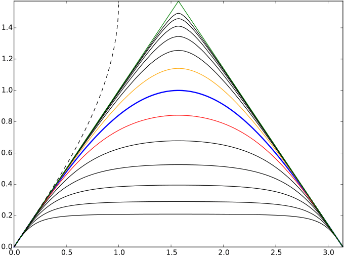
Iterates of the sine function (blue), in the first half-period. Half-iterate (orange), i.e., the sine's functional square root; the functional square root of that, the quarter-iterate (black) above it, and further fractional iterates up to the 1/64th. The functions below sine are six integral iterates below it, starting with the second iterate (red) and ending with the 64th iterate. The green envelope triangle represents the limiting null iterate, the sawtooth function serving as the starting point leading to the sine function. The dashed line is the negative first iterate, i.e. the inverse of sine (arcsin).
- sin[2](x) = sin(sin(x)) [red curve]
- sin[1](x) = sin(x) = rin(rin(x)) [blue curve]
- sin[½](x) = rin(x) = qin(qin(x)) [orange curve]
- sin[¼](x) = qin(x) [black curve above the orange curve]
- sin[–1](x) = arcsin(x) [dashed curve]
(Cf. the general pedagogy web-site.[6] For the notation, see .)
See also
References
- ↑ Kneser, H. (1950). "Reelle analytische Lösungen der Gleichung φ(φ(x)) = ex und verwandter Funktionalgleichungen". Journal für die reine und angewandte Mathematik. 187: 56&ndash, 67.
- ↑ Jeremy Gray and Karen Parshall (2007) Episodes in the History of Modern Algebra (1800–1950), American Mathematical Society, ISBN 978-0-8218-4343-7
- ↑ Schröder, E. (1870). "Ueber iterirte Functionen". Mathematische Annalen. 3 (2): 296&ndash, 322. doi:10.1007/BF01443992.
- ↑ Szekeres, G. (1958). "Regular iteration of real and complex functions". Acta Mathematica. 100 (3–4): 361–376. doi:10.1007/BF02559539.
- ↑ Curtright, T.; Zachos, C.; Jin, X. (2011). "Approximate solutions of functional equations". Journal of Physics A. 44 (40): 405205. arXiv:1105.3664. Bibcode:2011JPhA...44N5205C. doi:10.1088/1751-8113/44/40/405205.
- ↑ Curtright, T.L. Evolution surfaces and Schröder functional methods.
This article is issued from
Wikipedia.
The text is licensed under Creative Commons - Attribution - Sharealike.
Additional terms may apply for the media files.