Asynchronous circuit

An asynchronous circuit, or self-timed circuit, is a sequential digital logic circuit which is not governed by a clock circuit or global clock signal. Instead it often uses signals that indicate completion of instructions and operations, specified by simple data transfer protocols. This type of circuit is contrasted with synchronous circuits, in which changes to the signal values in the circuit are triggered by repetitive pulses called a clock signal. Most digital devices today use synchronous circuits. However asynchronous circuits have the potential to be faster, and may also have advantages in lower power consumption, lower electromagnetic interference, and better modularity in large systems. Asynchronous circuits are an active area of research in digital logic design.

Synchronous vs asynchronous logic

Digital logic circuits can be divided into combinational logic, in which the output signals depend only on the current input signals, and sequential logic, in which the output depends both on current input and on past inputs. In other words, sequential logic is combinational logic with memory. Virtually all practical digital devices require sequential logic. Sequential logic can be divided into two types, synchronous logic and asynchronous logic.

• In synchronous logic circuits, an electronic oscillator generates a repetitive series of equally spaced pulses called the clock signal. The clock signal is applied to all the memory elements in the circuit, called flip-flops. The output of the flip-flops only changes when triggered by the edge of the clock pulse, so changes to the logic signals throughout the circuit all begin at the same time, at regular intervals synchronized by the clock. The output of all memory elements in a circuit is called the state of the circuit. The state of a synchronous circuit changes only on the clock pulse. The changes in signal require a certain amount of time to propagate through the combinational logic gates of the circuit. This is called propagation delay. The period of the clock signal is made long enough so the output of all the logic gates have time to settle to stable values before the next clock pulse. As long as this condition is met, synchronous circuits will operate stably, so they are easy to design.

However a disadvantage of synchronous circuits is that they can be slow. The maximum possible clock rate is determined by the logic path with the longest propagation delay, called the critical path. So logic paths that complete their operations quickly are idle most of the time. Another problem is that the widely distributed clock signal takes a lot of power, and must run whether the circuit is receiving inputs or not.

• In asynchronous circuits, there is no clock signal, and the state of the circuit changes as soon as the inputs change. Since asynchronous circuits don't have to wait for a clock pulse to begin processing inputs, they can be faster than synchronous circuits, and their speed is theoretically limited only by the propagation delays of the logic gates. However, asynchronous circuits are more difficult to design and subject to problems not found in synchronous circuits. This is because the resulting state of an asynchronous circuit can be sensitive to the relative arrival times of inputs at gates. If transitions on two inputs arrive at almost the same time, the circuit can go into the wrong state depending on slight differences in the propagation delays of the gates. This is called a race condition. In synchronous circuits this problem is less severe because race conditions can only occur due to inputs from outside the synchronous system, called asynchronous inputs. Although some fully asynchronous digital systems have been built (see below), today asynchronous circuits are typically used in a few critical parts of otherwise synchronous systems where speed is at a premium, such as signal processing circuits.

Theoretical foundation

The term asynchronous logic is used to describe a variety of design styles, which use different assumptions about circuit properties.^[1] These vary from the bundled delay model – which uses "conventional" data processing elements with completion indicated by a locally generated delay model – to delay-insensitive design – where arbitrary delays through circuit elements can be accommodated. The latter style tends to yield circuits which are larger than bundled data implementations, but which are insensitive to layout and parametric variations and are thus "correct by design".

Asynchronous logic is the logic required for the design of asynchronous digital systems. These function without a clock signal and so individual logic elements cannot be relied upon to have a discrete true/false state at any given time. Boolean logic is inadequate for this and so extensions are required. Karl Fant developed a theoretical treatment of this in his work Logically determined design in 2005 which used four-valued logic with null and intermediate being the additional values. This architecture is important because it is quasi-delay-insensitive.^[2] Scott Smith and Jia Di developed an ultra-low-power variation of Fant's Null Convention Logic that incorporates multi-threshold CMOS.^[3] This variation is termed Multi-threshold Null Convention Logic (MTNCL), or alternatively Sleep Convention Logic (SCL).^[4] Vadim Vasyukevich developed a different approach based upon a new logical operation which he called venjunction. This takes into account not only the current value of an element, but also its history.^[5]

Petri nets are an attractive and powerful model for reasoning about asynchronous circuits. However, Petri nets have been criticized for their lack of physical realism (see Petri net: Subsequent models of concurrency). Subsequent to Petri nets other models of concurrency have been developed that can model asynchronous circuits including the Actor model and process calculi.

Benefits

A variety of advantages have been demonstrated by asynchronous circuits, including both quasi-delay-insensitive (QDI) circuits (generally agreed to be the most "pure" form of asynchronous logic that retains computational universality) and less pure forms of asynchronous circuitry which use timing constraints for higher performance and lower area and power:

• Robust handling of metastability of arbiters.
• Higher performance function units, which provide average-case (i.e. data-dependent) completion rather than worst-case completion. Examples include speculative completion^[6][7] which has been applied to design parallel prefix adders faster than synchronous ones, and a high-performance double-precision floating point adder'^[8] which outperforms leading synchronous designs.
• Early completion of a circuit when it is known that the inputs which have not yet arrived are irrelevant.
• Lower power consumption because no transistor ever transitions unless it is performing useful computation. Epson has reported 70% lower power consumption compared to synchronous design.^[9] Also, clock drivers can be removed which can significantly reduce power consumption. However, when using certain encodings, asynchronous circuits may require more area, which can result in increased power consumption if the underlying process has poor leakage properties (for example, deep submicrometer processes used prior to the introduction of High-k dielectrics).
• "Elastic" pipelines, which achieve high performance while gracefully handling variable input and output rates and mismatched pipeline stage delays.^[10]
• Freedom from the ever-worsening difficulties of distributing a high-fan-out, timing-sensitive clock signal.
• Better modularity and composability.
• Far fewer assumptions about the manufacturing process are required (most assumptions are timing assumptions).
• Circuit speed adapts to changing temperature and voltage conditions rather than being locked at the speed mandated by worst-case assumptions.
• Immunity to transistor-to-transistor variability in the manufacturing process, which is one of the most serious problems facing the semiconductor industry as dies shrink.
• Less severe electromagnetic interference (EMI). Synchronous circuits create a great deal of EMI in the frequency band at (or very near) their clock frequency and its harmonics; asynchronous circuits generate EMI patterns which are much more evenly spread across the spectrum.
• In asynchronous circuits, local signaling eliminates the need for global synchronization which exploits some potential advantages in comparison with synchronous ones. They have shown potential specifications in low power consumption, design reuse, improved noise immunity and electromagnetic compatibility. Asynchronous circuits are more tolerant to process variations and external voltage fluctuations.
• Less stress on the power distribution network. Synchronous circuits tend to draw a large amount of current right at the clock edge and shortly thereafter. The number of nodes switching (and thence, amount of current drawn) drops off rapidly after the clock edge, reaching zero just before the next clock edge. In an asynchronous circuit, the switching times of the nodes are not correlated in this manner, so the current draw tends to be more uniform and less bursty.

Disadvantages

• Area overhead may be up to double the number of circuit elements (transistors), due to addition of completion detection and design-for-test circuits.^[11]
• Fewer people are trained in this style compared to synchronous design.^[11]
• Synchronous designs are inherently easier to test and debug than asynchronous designs.^[12] However, this position is disputed by Fant, who claims that the apparent simplicity of synchronous logic is an artifact of the mathematical models used by the common design approaches.^[13]
• Clock gating in more conventional synchronous designs is an approximation of the asynchronous ideal, and in some cases, its simplicity may outweigh the advantages of a fully asynchronous design.
• Performance (speed) of asynchronous circuits may be reduced in architectures that require input-completeness (more complex data path).^[14]
• Lack of dedicated, asynchronous design-focused commercial EDA tools.^[14]

Communication

There are several ways to create asynchronous communication channels that can be classified by their protocol and data encoding.

Protocols

There are two widely used protocol families which differ in the way communications are encoded:

• two-phase handshake (a.k.a. two-phase protocol, Non-Return-to-Zero (NRZ) encoding, or transition signalling): Communications are represented by any wire transition; transitions from 0 to 1 and from 1 to 0 both count as communications.
• four-phase handshake (a.k.a. four-phase protocol, or Return-to-Zero (RZ) encoding): Communications are represented by a wire transition followed by a reset; a transition sequence from 0 to 1 and back to 0 counts as single communication.

Illustration of two and four-phase handshakes. Top: A sender and a receiver are communicating with simple request and acknowledge signals. The sender drives the request line, and the receiver drives the acknowledge line. Middle: Timing diagram of two, two-phase communications. Bottom: Timing diagram of one, four-phase communication.

Despite involving more transitions per communication, circuit implementations four-phase protocols are usually faster and simpler than two-phase protocols because the signal lines return to their original state by the end of each communication. In two-phase protocols, the circuit implementations would have to store the state of the signal line internally.

Note that these basic distinctions do not account for the wide variety of protocols. These protocols may encode only requests and acknowledgements or also encode the data, which leads to the popular multi-wire data encoding. Many other, less common protocols have been proposed including using a single wire for request and acknowledgment, using several significant voltages, using only pulses or balancing timings in order to remove the latches.

Data encoding

There are two widely used data encodings in asynchronous circuits: bundled-data encoding and multi-rail encoding

Another common way to encode the data is to use multiple wires to encode a single digit: the value is determined by the wire on which the event occurs. This avoids some of the delay assumptions necessary with bundled-data encoding, since the request and the data are not separated anymore.

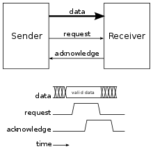
Bundled-data encoding

Bundled-data encoding uses one wire per bit of data with a request and an acknowledge signal; this is the same encoding used in synchronous circuits without the restriction that transitions occur on with a clock edge. The request and the acknowledge are sent on separate wires with one of the above protocols. These circuits usually assume a bounded delay model with the completion signals delayed long enough for the calculations to take place.

In operation, the sender signals the availability and validity of data with a request. The receiver then indicates completion with an acknowledgement, indicating that it is able to process new requests. That is, the request is bundled with the data, hence the name "bundled-data".

Bundled-data circuits are often referred to as micropipelines, whether they use a two-phase or four-phase protocol, even if the term was initially introduced for two-phase bundled-data.

A 4-phase, bundled-data communication. Top: A sender and receiver are connected by data lines, a request line, and an acknowledge line. Bottom: Timing diagram of a bundled data communication. When the request line is low, the data is to be considered invalid and liable to change at anytime.

Multi-rail encoding

Multi-rail encoding uses multiple wires without a one-to-one relationship between bits and wires and a separate acknowledge signal. Data availability is indicated by the transitions themselves on one or more of the data wires (depending on the type of multi-rail encoding) instead of with a request signal as in the bundled-data encoding. This provides the advantage that the data communication is delay-insensitive. Two common multi-rail encodings are one-hot and dual rail. The one-hot (a.k.a. 1-of-n) encoding represents a number in base n with a communication on one of the n wires. The dual-rail encoding uses pairs of wires to represent each bit of the data, hence the name "dual-rail"; one wire in the pair represents the bit value of 0 and the other represents the bit value of 1. For example, a dual-rail encoded two bit number will be represented with two pairs of wires for four wires in total. During a data communication, communications occur on one of each pair of wires to indicate the data's bits. In the general case, an m n encoding represent data as m words of base n.

Diagram of dual rail and 1-of-4 communications. Top: A sender and receiver are connected by data lines and an acknowledge line. Middle: Timing diagram of the sender communicating the values 0, 1, 2, and then 3 to the receiver with the 1-of-4 encoding. Bottom: Timing diagram of the sender communicating the same values to the receiver with the dual-rail encoding. For this particular data size, the dual rail encoding is the same as a 2x1-of-2 encoding.

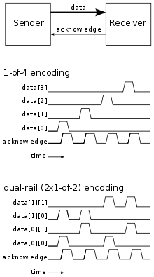
Dual-rail encoding with a four-phase protocol is the most common and is also called three-state encoding, since it has two valid states (10 and 01, after a transition) and a reset state (00). Another common encoding, which leads to a simpler implementation than one-hot, two-phase dual-rail is four-state encoding, or level-encoded dual-rail, and uses a data bit and a parity bit to achieve a two-phase protocol.

Asynchronous CPU

Asynchronous CPUs are one of several ideas for radically changing CPU design.

Unlike a conventional processor, a clockless processor (asynchronous CPU) has no central clock to coordinate the progress of data through the pipeline. Instead, stages of the CPU are coordinated using logic devices called "pipeline controls" or "FIFO sequencers." Basically, the pipeline controller clocks the next stage of logic when the existing stage is complete. In this way, a central clock is unnecessary. It may actually be even easier to implement high performance devices in asynchronous, as opposed to clocked, logic:

• components can run at different speeds on an asynchronous CPU; all major components of a clocked CPU must remain synchronized with the central clock;
• a traditional CPU cannot "go faster" than the expected worst-case performance of the slowest stage/instruction/component. When an asynchronous CPU completes an operation more quickly than anticipated, the next stage can immediately begin processing the results, rather than waiting for synchronization with a central clock. An operation might finish faster than normal because of attributes of the data being processed (e.g., multiplication can be very fast when multiplying by 0 or 1, even when running code produced by a naive compiler), or because of the presence of a higher voltage or bus speed setting, or a lower ambient temperature, than 'normal' or expected.

Asynchronous logic proponents believe these capabilities would have these benefits:

• lower power dissipation for a given performance level, and
• highest possible execution speeds.

The biggest disadvantage of the clockless CPU is that most CPU design tools assume a clocked CPU (i.e., a synchronous circuit). Many tools "enforce synchronous design practices".^[15] Making a clockless CPU (designing an asynchronous circuit) involves modifying the design tools to handle clockless logic and doing extra testing to ensure the design avoids metastable problems. The group that designed the AMULET, for example, developed a tool called LARD^[16] to cope with the complex design of AMULET3.

Despite the difficulty of doing so, numerous asynchronous CPUs have been built, including:

• the ORDVAC and the (identical) ILLIAC I (1951)^[17][18]
• the Johnniac (1953)^[19]
• the WEIZAC (1955)
• the ILLIAC II (1962)^[17]
• The Victoria University of Manchester built Atlas (1964)
• The ICL 1906A and 1906S mainframe computers, part of the 1900 series and sold from 1964 for over a decade by ICL ^[20]
• The Honeywell CPUs 6180 (1972)^[21] and Series 60 Level 68 (1981)^[22][23] upon which Multics ran asynchronously
• Soviet bit-slice microprocessor modules (late 1970s) ^[24][25] produced as К587,^[26] К588^[27] and К1883 (U83x in East Germany)^[28]
• The Caltech Asynchronous Microprocessor, the world-first asynchronous microprocessor (1988);
• the ARM-implementing AMULET (1993 and 2000);
• the asynchronous implementation of MIPS R3000, dubbed MiniMIPS (1998);
• several versions of the XAP processor experimented with different asynchronous design styles: a bundled data XAP, a 1-of-4 XAP, and a 1-of-2 (dual-rail) XAP (2003?);^[29]
• an ARM-compatible processor (2003?) designed by Z. C. Yu, S. B. Furber, and L. A. Plana; "designed specifically to explore the benefits of asynchronous design for security sensitive applications";^[29]
• the "Network-based Asynchronous Architecture" processor (2005) that executes a subset of the MIPS architecture instruction set;^[29]
• the ARM996HS processor (2006) from Handshake Solutions
• the HT80C51 processor (2007?) from Handshake Solutions^[30]
• the SEAforth multi-core processor (2008) from Charles H. Moore.^[31]
• the GA144^[32] multi-core processor (2010) from Charles H. Moore.
• TAM16: 16-bit asynchronous microcontroller IP core (Tiempo) ^[33]

The ILLIAC II was the first completely asynchronous, speed independent processor design ever built; it was the most powerful computer at the time.^[17]

DEC PDP-16 Register Transfer Modules (ca. 1973) allowed the experimenter to construct asynchronous, 16-bit processing elements. Delays for each module were fixed and based on the module's worst-case timing.

The Caltech Asynchronous Microprocessor (1988) was the first asynchronous microprocessor (1988). Caltech designed and manufactured the world's first fully Quasi Delay Insensitive processor. During demonstrations, the researchers loaded a simple program which ran in a tight loop, pulsing one of the output lines after each instruction. This output line was connected to an oscilloscope. When a cup of hot coffee was placed on the chip, the pulse rate (the effective "clock rate") naturally slowed down to adapt to the worsening performance of the heated transistors. When liquid nitrogen was poured on the chip, the instruction rate shot up with no additional intervention. Additionally, at lower temperatures, the voltage supplied to the chip could be safely increased, which also improved the instruction rate – again, with no additional configuration.

In 2004, Epson manufactured the world's first bendable microprocessor called ACT11, an 8-bit asynchronous chip.^{[34][35][36][37][38]} Synchronous flexible processors are slower, since bending the material on which a chip is fabricated causes wild and unpredictable variations in the delays of various transistors, for which worst-case scenarios must be assumed everywhere and everything must be clocked at worst-case speed. The processor is intended for use in smart cards, whose chips are currently limited in size to those small enough that they can remain perfectly rigid.

In 2014, IBM announced a SyNAPSE-developed chip that runs in an asynchronous manner, with one of the highest transistor counts of any chip ever produced. IBM's chip consumes orders of magnitude less power than traditional computing systems on pattern recognition benchmarks.^[39]

See also

• Sequential logic (asynchronous)
• Asynchrobatic logic
• Perfect clock gating

References

Further reading

• TiDE from Handshakesolutions in The Netherlands, Commercial asynchronous circuits design tool. Commercial asynchronous ARM(ARM996HS) and 8051(HT80C51) are available.
• S. M. Nowick and M. Singh, High-Performance Asynchronous Pipelines: an Overview, IEEE Design and Test of Computers, special issue on asynchronous design, vol. 28:5, pp. 8–22 (September/October 2011). Provides a good basic introduction to asynchronous design, handshaking protocols, data encoding techniques, industrial developments, as well as a technical overview of several leading high-performance pipelines, and their recent use at Intel, Achronix Semiconductor, and other companies.
• An introduction to asynchronous circuit design by Davis and Nowick
• Asynchronous logic elements. Venjunction and sequention by V. O. Vasyukevich
• Null convention logic, a design style pioneered by Theseus Logic, who have fabricated over 20 ASICs based on their NCL08 and NCL8501 microcontroller cores
• The Status of Asynchronous Design in Industry Information Society Technologies (IST) Programme, IST-1999-29119, D. A. Edwards W. B. Toms, June 2004, via www.scism.lsbu.ac.uk
• The Red Star is a version of the MIPS R3000 implemented in asynchronous logic
• The Amulet microprocessors were asynchronous ARMs, built in the 1990s at University of Manchester, England
• The N-Protocol developed by Navarre AsyncArt, the first commercial asynchronous design methodology for conventional FPGAs.
• PGPSALM an asynchronous implementation of the 6502 microprocessor
• Caltech Async Group home page
• Tiempo: French company providing asynchronous IP and design tools
• Epson ACT11 Flexible CPU Press Release

References

- ↑ van Berkel, C. H. and M. B. Josephs and S. M. Nowick (February 1999), "Applications of Asynchronous Circuits" (PDF), Proceedings of the IEEE, 87 (2): 234–242, doi:10.1109/5.740016
- ↑ Karl M. Fant (2005), Logically determined design: clockless system design with NULL convention logic (NCL), John Wiley and Sons, ISBN 978-0-471-68478-7
- ↑ Smith, Scott and Di, Jia (2009). Designing Asynchronous Circuits using NULL Conventional Logic (NCL). Morgan & Claypool Publishers. ISBN 978-1-59829-981-6.
- ↑ Scott, Smith and Di, Jia. "U.S. 7,977,972 Ultra-Low Power Multi-threshold Asychronous Circuit Design". Retrieved 2011-12-12.
- ↑ Vasyukevich, V. O. (April 2007), "Decoding asynchronous sequences", Automatic Control and Computer Sciences, Allerton Press, 41 (2): 93–99, doi:10.3103/S0146411607020058, ISSN 1558-108X
- ↑ Nowick, S. M. and K. Y. Yun and P. A. Beerel and A. E. Dooply (March 1997), "Speculative Completion for the Design of High-Performance Asynchronous Dynamic Adders" (PDF), Proceedings of the IEEE International Symposium on Advanced Research in Asynchronous Circuits and Systems ('Async'): 210–223
- ↑ Nowick, S. M. (September 1996), "Design of a Low-Latency Asynchronous Adder Using Speculative Completion" (PDF), IEE Proceedings -- Computers and Digital Techniques: 301–307
- ↑ Sheikh, B. and R. Manohar (May 2010), "An Operand-Optimized Asynchronous IEEE 754 Double-Precision Floating-Point Adder" (PDF), Proceedings of the IEEE International Symposium on Asynchronous Circuits and Systems ('Async'): 151–162
- ↑ "Epson Develops the World's First Flexible 8-Bit Asynchronous Microprocessor" 2005
- ↑ Nowick, S. M. and M. Singh (Sep–Oct 2011), "High-Performance Asynchronous Pipelines: an Overview" (PDF), IEEE Design & Test of Computers, special issue on asynchronous design, 28 (5): 8–22, doi:10.1109/mdt.2011.71
- 1 2 Furber, Steve. "Principles of Asynchronous Circuit Design" (PDF). Pg. 232. Archived from the original (PDF) on 2012-04-26. Retrieved 2011-12-13.
- ↑ "Keep It Strictly Synchronous: KISS those asynchronous-logic problems good-bye". Personal Engineering and Instrumentation News, November 1997, pages 53–55. http://www.fpga-site.com/kiss.html
- ↑ Karl M. Fant (2007), Computer Science Reconsidered: The Invocation Model of Process Expression, John Wiley and Sons, ISBN 978-0471798149
- 1 2 van Leeuwen, T. M. (2010). Implementation and automatic generation of asynchronous scheduled dataflow graph. Delft.
- ↑ "ASIC to FPGA migration"
- ↑ LARD Archived March 6, 2005, at the Wayback Machine.
- 1 2 3 "In the 1950 and 1960s, asynchronous design was used in many early mainframe computers, including the ILLIAC I and ILLIAC II ... ." Brief History of asynchronous circuit design
- ↑ "The Illiac is a binary parallel asynchronous computer in which negative numbers are represented as two's complements." – final summary of "Illiac Design Techniques" 1955.
- ↑ Johnniac history written in 1968
- ↑
- ↑ "Entirely asynchronous, its hundred-odd boards would send out requests, earmark the results for somebody else, swipe somebody else's signals or data, and backstab each other in all sorts of amusing ways which occasionally failed (the "op not complete" timer would go off and cause a fault). ... [There] was no hint of an organized synchronization strategy: various "it's ready now", "ok, go", "take a cycle" pulses merely surged through the vast backpanel ANDed with appropriate state and goosed the next guy down. Not without its charms, this seemingly ad-hoc technology facilitated a substantial degree of overlap ... as well as the [segmentation and paging] of the Multics address mechanism to the extant 6000 architecture in an ingenious, modular, and surprising way ... . Modification and debugging of the processor, though, were no fun." "Multics Glossary: ... 6180"
- ↑ "10/81 ... DPS 8/70M CPUs" Multics Chronology
- ↑ "The Series 60, Level 68 was just a repackaging of the 6180." Multics Hardware features: Series 60, Level 68
- ↑ A. A. Vasenkov, V. L. Dshkhunian, P. R. Mashevich, P. V. Nesterov, V. V. Telenkov, Ju. E. Chicherin, D. I. Juditsky, "Microprocessor computing system," Patent US4124890, Nov. 7, 1978
- ↑ Chapter 4.5.3 in the biography of D. I. Juditsky (in Russian)
- ↑ "Archived copy". Archived from the original on 2015-07-17. Retrieved 2015-07-16.
- ↑ "Archived copy". Archived from the original on 2015-07-22. Retrieved 2015-07-19.
- 1 2 3 "A Network-based Asynchronous Architecture for Cryptographic Devices" by Ljiljana Spadavecchia 2005 in section "4.10.2 Side-channel analysis of dual-rail asynchronous architectures" and section "5.5.5.1 Instruction set"
- ↑ "Handshake Solutions HT80C51" "The Handshake Solutions HT80C51 is a Low power, asynchronous 80C51 implementation using handshake technology, compatible with the standard 8051 instruction set."
- ↑ SEAforth Overview Archived 2008-02-02 at the Wayback Machine. "... asynchronous circuit design throughout the chip. There is no central clock with billions of dumb nodes dissipating useless power. ... the processor cores are internally asynchronous themselves."
- ↑ "GreenArrayChips" "Ultra-low-powered multi-computer chips with integrated peripherals."
- ↑ Tiempo: Asynchronous TAM16 Core IP
- ↑ "Seiko Epson tips flexible processor via TFT technology" by Mark LaPedus 2005
- ↑ "A flexible 8b asynchronous microprocessor based on low-temperature poly-silicon TFT technology" by Karaki et al. 2005. Abstract: "A flexible 8b asynchronous microprocessor ACTII ... The power level is 30% of the synchronous counterpart."
- ↑ "Introduction of TFT R&D Activities in Seiko Epson Corporation" by Tatsuya Shimoda (2005?) has picture of "A flexible 8-bit asynchronous microprocessor, ACT11"
- ↑ "Epson Develops the World's First Flexible 8-Bit Asynchronous Microprocessor"
- ↑ "Seiko Epson details flexible microprocessor: A4 sheets of e-paper in the pipeline by Paul Kallender 2005
- ↑ "SyNAPSE program develops advanced brain-inspired chip" Archived 2014-08-10 at the Wayback Machine.. August 07, 2014.