AVL tree

AVL tree
Type	tree
Invented	1962
Invented by	Georgy Adelson-Velsky and Evgenii Landis
Time complexity in big O notation

Animation showing the insertion of several elements into an AVL tree. It includes left, right, left-right and right-left rotations.

Fig. 1: AVL tree with balance factors (green)

In computer science, an AVL tree (named after inventors Adelson-Velsky and Landis) is a self-balancing binary search tree. It was the first such data structure to be invented.^[2] In an AVL tree, the heights of the two child subtrees of any node differ by at most one; if at any time they differ by more than one, rebalancing is done to restore this property. Lookup, insertion, and deletion all take $O (log n)$ time in both the average and worst cases, where $n$ is the number of nodes in the tree prior to the operation. Insertions and deletions may require the tree to be rebalanced by one or more tree rotations.

The AVL tree is named after its two Soviet inventors, Georgy Adelson-Velsky and Evgenii Landis, who published it in their 1962 paper "An algorithm for the organization of information".^[3]

AVL trees are often compared with red–black trees because both support the same set of operations and take $O(\log n)$ time for the basic operations. For lookup-intensive applications, AVL trees are faster than red–black trees because they are more strictly balanced.^[4] Similar to red–black trees, AVL trees are height-balanced. Both are, in general, neither weight-balanced nor $\mu$ -balanced for any $\mu \leq {\frac {1}{2}}$ ^[5] that is, sibling nodes can have hugely differing numbers of descendants.

Definition

Balance factor

In a binary tree the balance factor of a node N is defined to be the height difference

BalanceFactor(

N

) : = Height(RightSubtree(

N

)) - Height(LeftSubtree(

N

))

^[6]

of its two child subtrees. A binary tree is defined to be an AVL tree if the invariant

BalanceFactor(

N

) \in {-1,0,+1

}^[7]

holds for every node N in the tree.

A node N with $BalanceFactor($ N $) < 0$ is called "left-heavy", one with $BalanceFactor($ N $) > 0$ is called "right-heavy", and one with $BalanceFactor($ N $) = 0$ is sometimes simply called "balanced".

Remark

In what follows, because there is a one-to-one correspondence between nodes and the subtrees rooted by them, the name of an object is sometimes used to refer to the node and sometimes used to refer to the subtree.

Properties

Balance factors can be kept up-to-date by knowing the previous balance factors and the change in height – it is not necessary to know the absolute height. For holding the AVL balance information in the traditional way, two bits per node are sufficient. However, later research showed if the AVL tree is implemented as a rank balanced tree with delta ranks allowed of 1 or 2 – with meaning "when going upward there is an additional increment in height of one or two", this can be done with one bit.

The height $h$ of an AVL tree with $n$ nodes lies in the interval:^[8]

\log _{2}(n+1)\leq h<c\log _{2}(n+2)+b

with the golden ratio $φ : = (1+$ √ $5$ $) ⁄ 2 \approx 1.618$ , $c : = 1 ⁄ log 2 φ \approx 1.44$ , and $b : = c ⁄ 2 log 2 5 - 2 \approx -0.328$ . This is because an AVL tree of height $h$ contains at least $F h +2 - 1$ nodes where ${F h}$ is the Fibonacci sequence with the seed values $F 1 = 1$ , $F 2 = 1$ .

Operations

Read-only operations of an AVL tree involve carrying out the same actions as would be carried out on an unbalanced binary search tree, but modifications have to observe and restore the height balance of the subtrees.

Searching

Searching for a specific key in an AVL tree can be done the same way as that of a normal unbalanced binary search tree. In order for search to work effectively it has to employ a comparison function which establishes a total order (or at least a total preorder) on the set of keys. The number of comparisons required for successful search is limited by the height $h$ and for unsuccessful search is very close to $h$ , so both are in $O(log n)$ .

Traversal

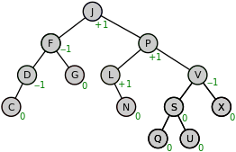
Once a node has been found in an AVL tree, the next or previous node can be accessed in amortized constant time. Some instances of exploring these "nearby" nodes require traversing up to $h \propto log(n)$ links (particularly when navigating from the rightmost leaf of the root’s left subtree to the root or from the root to the leftmost leaf of the root’s right subtree; in the AVL tree of figure 1, moving from node P to the next but one node Q takes 3 steps). However, exploring all $n$ nodes of the tree in this manner would visit each link exactly twice: one downward visit to enter the subtree rooted by that node, another visit upward to leave that node’s subtree after having explored it. And since there are $n -1$ links in any tree, the amortized cost is $2\times(n -1)/ n$ , or approximately 2.

Insert

When inserting an element into an AVL tree, you initially follow the same process as inserting into a Binary Search Tree. More explicitly: In case a preceding search has not been successful the search routine returns the tree itself with indication EMPTY and the new node is inserted as root. Or, if the tree has not been empty the search routine returns a node and a direction (left or right) where the returned node does not have a child. Then the node to be inserted is made child of the returned node at the returned direction.

After this insertion it is necessary to check each of the node’s ancestors for consistency with the invariants of AVL trees: this is called "retracing". This is achieved by considering the balance factor of each node.^[9]^[10]

Since with a single insertion the height of an AVL subtree cannot increase by more than one, the temporary balance factor of a node after an insertion will be in the range [–2,+2]. For each node checked, if the temporary balance factor remains in the range from –1 to +1 then only an update of the balance factor and no rotation is necessary. However, if the temporary balance factor becomes less than –1 or greater than +1, the subtree rooted at this node is AVL unbalanced, and a rotation is needed. The various cases of rotations are described in section Rebalancing.

In figure 1, by inserting the new node Z as a child of node X the height of that subtree Z increases from 0 to 1.

Invariant of the retracing loop for an insertion

The height of the subtree rooted by Z has increased by 1. It is already in AVL shape.

 1 for (X = parent(Z); X != null; X = parent(Z)) { // Loop (possibly up to the root)
 2     // BalanceFactor(X) has to be updated:
 3     if (Z == right_child(X)) { // The right subtree increases
 4         if (BalanceFactor(X) > 0) { // X is right-heavy
 5             // ===> the temporary BalanceFactor(X) == +2
 6             // ===> rebalancing is required.
 7             G = parent(X); // Save parent of X around rotations
 8             if (BalanceFactor(Z) < 0)      // Right Left Case     (see figure 5)
 9                 N = rotate_RightLeft(X, Z); // Double rotation: Right(Z) then Left(X)
10             else                           // Right Right Case    (see figure 4)
11                 N = rotate_Left(X, Z);     // Single rotation Left(X)
12             // After rotation adapt parent link
13         } else {
14             if (BalanceFactor(X) < 0) {
15                 BalanceFactor(X) = 0; // Z’s height increase is absorbed at X.
16                 break; // Leave the loop
17             }
18             BalanceFactor(X) = +1;
19             Z = X; // Height(Z) increases by 1
20             continue;
21         }
22     } else { // Z == left_child(X): the left subtree increases
23         if (BalanceFactor(X) < 0) { // X is left-heavy
24             // ===> the temporary BalanceFactor(X) == –2
25             // ===> rebalancing is required.
26             G = parent(X); // Save parent of X around rotations
27             if (BalanceFactor(Z) > 0)      // Left Right Case
28                 N = rotate_LeftRight(X, Z); // Double rotation: Left(Z) then Right(X)
29             else                           // Left Left Case
30                 N = rotate_Right(X, Z);    // Single rotation Right(X)
31             // After rotation adapt parent link
32         } else {
33             if (BalanceFactor(X) > 0) {
34                 BalanceFactor(X) = 0; // Z’s height increase is absorbed at X.
35                 break; // Leave the loop
36             }
37             BalanceFactor(X) = –1;
38             Z = X; // Height(Z) increases by 1
39             continue;
40         }
41     }
42     // After a rotation adapt parent link:
43     // N is the new root of the rotated subtree
44     // Height does not change: Height(N) == old Height(X)
45     parent(N) = G;
46     if (G != null) {
47         if (X == left_child(G))
48             left_child(G) = N;
49         else
50             right_child(G) = N;
51         break;
52     } else {
53         tree->root = N; // N is the new root of the total tree
54         break;
55     }
56     // There is no fall thru, only break; or continue;
57 }
58 // Unless loop is left via break, the height of the total tree increases by 1.

In order to update the balance factors of all nodes, first observe that all nodes requiring correction lie from child to parent along the path of the inserted leaf. If the above procedure is applied to nodes along this path, starting from the leaf, then every node in the tree will again have a balance factor of −1, 0, or 1.

The retracing can stop if the balance factor becomes 0 implying that the height of that subtree remains unchanged.

If the balance factor becomes ±1 then the height of the subtree increases by one and the retracing needs to continue.

If the balance factor temporarily becomes ±2, this has to be repaired by an appropriate rotation after which the subtree has the same height as before (and its root the balance factor 0).

The time required is $O(log n)$ for lookup, plus a maximum of $O(log n)$ retracing levels ( $O(1)$ on average) on the way back to the root, so the operation can be completed in $O(log n)$ time.

Delete

The preliminary steps for deleting a node are described in section Binary search tree#Deletion. There, the effective deletion of the subject node or the replacement node decreases the height of the corresponding child tree either from 1 to 0 or from 2 to 1, if that node had a child.

Starting at this subtree, it is necessary to check each of the ancestors for consistency with the invariants of AVL trees. This is called "retracing".

Since with a single deletion the height of an AVL subtree cannot decrease by more than one, the temporary balance factor of a node will be in the range from −2 to +2. If the balance factor remains in the range from −1 to +1 it can be adjusted in accord with the AVL rules. If it becomes ±2 then the subtree is unbalanced and needs to be rotated. The various cases of rotations are described in section Rebalancing.

Invariant of the retracing loop for a deletion

The height of the subtree rooted by N has decreased by 1. It is already in AVL shape.

 1 for (X = parent(N); X != null; X = G) { // Loop (possibly up to the root)
 2     G = parent(X); // Save parent of X around rotations
 3     // BalanceFactor(X) has not yet been updated!
 4     if (N == left_child(X)) { // the left subtree decreases
 5         if (BalanceFactor(X) > 0) { // X is right-heavy
 6             // ===> the temporary BalanceFactor(X) == +2
 7             // ===> rebalancing is required.
 8             Z = right_child(X); // Sibling of N (higher by 2)
 9             b = BalanceFactor(Z);
10             if (b < 0)                     // Right Left Case     (see figure 5)
11                 N = rotate_RightLeft(X, Z); // Double rotation: Right(Z) then Left(X)
12             else                           // Right Right Case    (see figure 4)
13                 N = rotate_Left(X, Z);     // Single rotation Left(X)
14             // After rotation adapt parent link
15         } else {
16             if (BalanceFactor(X) == 0) {
17                 BalanceFactor(X) = +1; // N’s height decrease is absorbed at X.
18                 break; // Leave the loop
19             }
20             N = X;
21             BalanceFactor(N) = 0; // Height(N) decreases by 1
22             continue;
23         }
24     } else { // (N == right_child(X)): The right subtree decreases
25         if (BalanceFactor(X) < 0) { // X is left-heavy
26             // ===> the temporary BalanceFactor(X) == –2
27             // ===> rebalancing is required.
28             Z = left_child(X); // Sibling of N (higher by 2)
29             b = BalanceFactor(Z);
30             if (b > 0)                     // Left Right Case
31                 N = rotate_LeftRight(X, Z); // Double rotation: Left(Z) then Right(X)
32             else                        // Left Left Case
33                 N = rotate_Right(X, Z);    // Single rotation Right(X)
34             // After rotation adapt parent link
35         } else {
36             if (BalanceFactor(X) == 0) {
37                 BalanceFactor(X) = –1; // N’s height decrease is absorbed at X.
38                 break; // Leave the loop
39             }
40             N = X;
41             BalanceFactor(N) = 0; // Height(N) decreases by 1
42             continue;
43         }
44     }
45     // After a rotation adapt parent link:
46     // N is the new root of the rotated subtree
47     parent(N) = G;
48     if (G != null) {
49         if (X == left_child(G))
50             left_child(G) = N;
51         else
52             right_child(G) = N;
53         if (b == 0)
54             break; // Height does not change: Leave the loop
55     } else {
56         tree->root = N; // N is the new root of the total tree
57     }
58     // Height(N) decreases by 1 (== old Height(X)-1)
59 }
60 // Unless loop is left via break, the height of the total tree decreases by 1.

The retracing can stop if the balance factor becomes ±1 meaning that the height of that subtree remains unchanged.

If the balance factor becomes 0 then the height of the subtree decreases by one and the retracing needs to continue.

If the balance factor temporarily becomes ±2, this has to be repaired by an appropriate rotation. It depends on the balance factor of the sibling Z (the higher child tree) whether the height of the subtree decreases by one or does not change (the latter, if Z has the balance factor 0).

The time required is $O(log n)$ for lookup, plus a maximum of $O(log n)$ retracing levels ( $O(1)$ on average) on the way back to the root, so the operation can be completed in $O(log n)$ time.

Set operations and bulk operations

In addition to the single-element insert, delete and lookup operations, several set operations have been defined on AVL trees: union, intersection and set difference. Then fast bulk operations on insertions or deletions can be implemented based on these set functions. These set operations rely on two helper operations, Split and Join. With the new operations, the implementation of AVL trees can be more efficient and highly-parallelizable.^[11]

Join: The function Join is on two AVL trees $t 1$ and $t 2$ and a key $k$ will return a tree containing all elements in $t 1$ , $t 2$ as well as $k$ . It requires $k$ to be greater than all keys in $t 1$ and smaller than all keys in $t 2$ . If the two trees differ by height at most one, Join simply create a new node with left subtree $t 1$ , root $k$ and right subtree $t 2$ . Otherwise, suppose that $t 1$ is higher than $t 2$ for more than one (the other case is symmetric). Join follows the right spine of $t 1$ until a node $c$ which is balanced with $t 2$ . At this point a new node with left child $c$ , root $k$ and right child $t 2$ is created to replace c. The new node satisfies the AVL invariant, and its height is one greater than $c$ . The increase in height can increase the height of its ancestors, possibly invalidating the AVL invariant of those nodes. This can be fixed either with a double rotation if invalid at the parent or a single left rotation if invalid higher in the tree, in both cases restoring the height for any further ancestor nodes. Join will therefore require at most two rotations. The cost of this function is the difference of the heights between the two input trees.
Split: To split an AVL tree into two smaller trees, those smaller than key x, and those larger than key x, first draw a path from the root by inserting x into the AVL. After this insertion, all values less than x will be found on the left of the path, and all values greater than x will be found on the right. By applying Join, all the subtrees on the left side are merged bottom-up using keys on the path as intermediate nodes from bottom to top to form the left tree, and the right part is asymmetric. The cost of Split is $O(\log n)$ , order of the height of the tree.

The join algorithm is as follows:

function joinRightAVL(T_L, k, T_R)
    (l,k',c)=expose(T_L)
    if (h(c)<h(T_R)+1)
       T'=Node(c,k,T_R)
       if (h(T')<=h(l)+1) then return Node(l,k',T')
       else return rotateLeft(Node(l,k'rotateRight(T')))
    else 
        T'=joinRightAVL(c,k,T_R)
        T=Node(l,k',T')
        if (h(T_L)>h(T_R)+1) return T
        else return rotateLeft(T)
function joinLeftAVL(T_L, k, T_R)
  /* symmetric to joinRightAVL */
function join(T_L, k, T_R)
    if (h(T_L)>h(T_R)+1) return joinRightAVL(T_L, k, T_R)
    if (h(T_R)>h(T_L)+1) return joinLeftAVL(T_L, k, T_R)
    return Node(T_L,k,T_R)

Here $h(v)$ of a node $v$ the height of $v$ . expose(v)=(l,k,r) means to extract a tree node $v$ 's left child $l$ , the key of the node $k$ , and the right child $r$ . Node(l,k,r) means to create a node of left child $l$ , key $k$ , and right child $r$ .

The split algorithm is as follows:

function split(T,k)
    if (T=nil) return (nil,false,nil)
    (L,(m,c),R)=expose(T)
    if (k=m) return (L,true,R)
    if (k<m) 
       (L',b,R')=split(L,k)
       return (L',b,join(R',m,R))
    if (k>m) 
       (L',b,R')=split(R,k)
       return (join(L,m,L'),b,R))

The union of two AVLs $t 1$ and $t 2$ representing sets $A$ and $B$ , is an AVL $t$ that represents $A \cup B$ . The following recursive function computes this union:

function union(t₁, t₂):
    if t₁ = nil:
        return t₂
    if t₂ = nil:
        return t₁
    t_<, t_> ← split t₂ on t₁.root
    return join(t₁.root,union(left(t₁), t_<),union(right(t₁), t_>))

Here, Split is presumed to return two trees: one holding the keys less its input key, one holding the greater keys. (The algorithm is non-destructive, but an in-place destructive version exists as well.)

The algorithm for intersection or difference is similar, but requires the Join2 helper routine that is the same as Join but without the middle key. Based on the new functions for union, intersection or difference, either one key or multiple keys can be inserted to or deleted from the AVL tree. Since Split calls Join but does not deal with the balancing criteria of AVL trees directly, such an implementation is usually called the "join-based" implementation.

The complexity of each of union, intersection and difference is $O\left(m\log \left({n \over m}+1\right)\right)$ for AVLs of sizes $m$ and $n(\geq m)$ . More importantly, since the recursive calls to union, intersection or difference are independent of each other, they can be executed in parallel with a parallel depth $O(\log m\log n)$ .^[11] When $m=1$ , the join-based implementation has the same computational DAG as single-element insertion and deletion.

Rebalancing

If during a modifying operation (e.g. insert, delete) a (temporary) height difference of more than one arises between two child subtrees, the parent subtree has to be "rebalanced". The given repair tools are the so-called tree rotations, because they move the keys only "vertically", so that the ("horizontal") in-order sequence of the keys is fully preserved (which is essential for a binary-search tree).^[9]^[10]

Let X be the node that has a (temporary) balance factor of −2 or +2. Its left or right subtree was modified. Let Z be the higher child. Note that Z is in AVL shape by induction hypothesis.

In case of insertion this insertion has happened to one of Z's children in a way that Z's height has increased. In case of deletion this deletion has happened to the sibling t₁ of Z in a way so that t₁'s height being already lower has decreased. (In that case Z's balance factor may be 0.)

There are four situations that might arise. We will describe them as Dir1 Dir2, where Dir1 comes from the set { left, right } and Dir2 as a balance factor comes from the set { left-heavy = −1, balanced = 0, right-heavy = +1 }.^[12]

Situation Dir1 Dir2 denotes:

Z is a Dir1 child of its parent and

Z is Dir2-heavy if Dir2 != Dir1

Z is not (−Dir2)-heavy if Dir2 == Dir1

i.e.

Right Right	=> Z is a right child of its parent X and	Z is not left-heavy	(i.e. BalanceFactor(Z) ≥ 0)	(see figure 4)
Left Left	=> Z is a left child of its parent X and	Z is not right-heavy	(i.e. BalanceFactor(Z) ≤ 0)
Right Left	=> Z is a right child of its parent X and	Z is left-heavy	(i.e. BalanceFactor(Z) = −1)	(see figure 5)
Left Right	=> Z is a left child of its parent X and	Z is right-heavy	(i.e. BalanceFactor(Z) = +1)

The balance violation of case Dir1 == Dir2 is repaired by a simple rotation rotate_(−Dir1) (rotate_Left in figure 4 resp. its mirror rotate_Right).

The case Dir1 != Dir2 is repaired by a double rotation rotate_(−Dir2)(−Dir1) == rotate_Dir1Dir2 (rotate_RightLeft in figure 5 resp. its mirror rotate_LeftRight).

The cost of a rotation, both simple and double, is constant.

Simple rotation

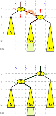
Figure 4 shows a Right Right situation. In its upper half, node X has two child trees with a balance factor of +2. Moreover, the inner child t₂₃ of Z (i.e., left child when Z is right child resp. right child when Z is left child) is not higher than its sibling t₄. This can happen by a height increase of subtree t₄ or by a height decrease of subtree t₁. In the latter case, also the pale situation where t₂₃ has the same height as t₄ may occur.

The result of the left rotation is shown in the lower half of the figure. Three links (thick edges in figure 4) and two balance factors are to be updated.

As the figure shows, before an insertion, the leaf layer was at level h+1, temporarily at level h+2 and after the rotation again at level h+1. In case of a deletion, the leaf layer was at level h+2, where it is again, when t₂₃ and t₄ were of same height. Otherwise the leaf layer reaches level h+1, so that the height of the rotated tree decreases.

Fig. 4: Simple rotation
rotate_Left(X,Z)

Code snippet of a simple left rotation

Input:	X = root of subtree to be rotated left
	Z = right child of X, Z is right-heavy
	with height == $Height(LeftSubtree($ X $))+2$
Result:	new root of rebalanced subtree

 1 node *rotate_Left(node *X, node *Z) {
 2     // Z is by 2 higher than its sibling
 3     t23 = left_child(Z); // Inner child of Z
 4     right_child(X) = t23;
 5     if (t23 != null)
 6         parent(t23) = X;
 7     left_child(Z) = X;
 8     parent(X) = Z;
 9     // 1st case, BalanceFactor(Z) == 0, only happens with deletion, not insertion:
10     if (BalanceFactor(Z) == 0) { // t23 has been of same height as t4
11         BalanceFactor(X) = +1;   // t23 now higher
12         BalanceFactor(Z) = –1;   // t4 now lower than X
13     } else { // 2nd case happens with insertion or deletion:
14         BalanceFactor(X) = 0;
15         BalanceFactor(Z) = 0;
16     }
17     return Z; // return new root of rotated subtree
18 }

Double rotation

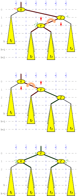
Figure 5 shows a Right Left situation. In its upper third, node X has two child trees with a balance factor of +2. But unlike figure 4, the inner child Y of Z is higher than its sibling t₄. This can happen by the insertion of Y itself or a height increase of one of its subtrees t₂ or t₃ (with the consequence that they are of different height) or by a height decrease of subtree t₁. In the latter case, it may also occur that t₂ and t₃ are of same height.

The result of the first, the right, rotation is shown in the middle third of the figure. (With respect to the balance factors, this rotation is not of the same kind as the other AVL single rotations, because the height difference between Y and t₄ is only 1.) The result of the final left rotation is shown in the lower third of the figure. Five links (thick edges in figure 5) and three balance factors are to be updated.

As the figure shows, before an insertion, the leaf layer was at level h+1, temporarily at level h+2 and after the double rotation again at level h+1. In case of a deletion, the leaf layer was at level h+2 and after the double rotation it is at level h+1, so that the height of the rotated tree decreases.

Fig. 5: Double rotation rotate_RightLeft(X,Z)
= rotate_Right around Z followed by
rotate_Left around X

Code snippet of a right-left double rotation

Input:	X = root of subtree to be rotated
	Z = its right child, left-heavy
	with height == $Height(LeftSubtree($ X $))+2$
Result:	new root of rebalanced subtree

 1 node *rotate_RightLeft(node *X, node *Z) {
 2     // Z is by 2 higher than its sibling
 3     Y = left_child(Z); // Inner child of Z
 4     // Y is by 1 higher than sibling
 5     t3 = right_child(Y);
 6     left_child(Z) = t3;
 7     if (t3 != null)
 8         parent(t3) = Z;
 9     right_child(Y) = Z;
10     parent(Z) = Y;
11     t2 = left_child(Y);
12     right_child(X) = t2;
13     if (t2 != null)
14         parent(t2) = X;
15     left_child(Y) = X;
16     parent(X) = Y;
17     if (BalanceFactor(Y) > 0) { // t3 was higher
18         BalanceFactor(X) = –1;  // t1 now higher
19         BalanceFactor(Z) = 0;
20     } else
21         if (BalanceFactor(Y) == 0) {
22             BalanceFactor(X) = 0;
23             BalanceFactor(Z) = 0;
24         } else {
25             // t2 was higher
26             BalanceFactor(X) = 0;
27             BalanceFactor(Z) = +1;  // t4 now higher
28         }
29     BalanceFactor(Y) = 0;
30     return Y; // return new root of rotated subtree
31 }

Comparison to other structures

Both AVL trees and red–black (RB) trees are self-balancing binary search trees and they are related mathematically. Indeed, every AVL tree can be colored red–black,^[13] but there are RB trees which are not AVL balanced. For maintaining the AVL resp. RB tree's invariants, rotations play an important role. In the worst case, even without rotations, AVL or RB insertions or deletions require $O(log n)$ inspections and/or updates to AVL balance factors resp. RB colors. RB insertions and deletions and AVL insertions require from zero to three tail-recursive rotations and run in amortized $O(1)$ time,^[14]^[15] thus equally constant on average. AVL deletions requiring $O(log n)$ rotations in the worst case are also $O(1)$ on average. RB trees require storing one bit of information (the color) in each node, while AVL trees mostly use two bits for the balance factor, although, when stored at the children, one bit with meaning «lower than sibling» suffices. The bigger difference between the two data structures is their height limit.

For a tree of size $n \geq 1$

an AVL tree’s height is at most
${\begin{array}{ll}h&\leqq \;c\log _{2}(n+d)+b\\&<\;c\log _{2}(n+2)+b\end{array}}$

where

\varphi :={\tfrac {1+{\sqrt {5}}}{2}}\approx 1.618

the golden ratio,

c:={\tfrac {1}{\log _{2}\varphi }}\approx 1.440,

b:={\tfrac {c}{2}}\log _{2}5-2\approx \;-0.328,

and

d:=1+{\tfrac {1}{\varphi ^{4}{\sqrt {5}}}}\approx 1.065

.

an RB tree’s height is at most
${\begin{array}{ll}h&\leqq \;2\log _{2}(n+1)\end{array}}$ .^[16]

AVL trees are more rigidly balanced than RB trees with an asymptotic relation ^AVL⁄_RB≈0.720 of the maximal heights. For insertions and deletions, Ben Pfaff shows in 79 measurements a relation of ^AVL⁄_RB between 0.677 and 1.077 with median ≈0.947 and geometric mean ≈0.910.^[17]

References

1 2 3 4 5 6 Eric Alexander. "AVL Trees".
↑ Robert Sedgewick, Algorithms, Addison-Wesley, 1983, ISBN 0-201-06672-6, page 199, chapter 15: Balanced Trees.
↑ Georgy Adelson-Velsky, G.; Evgenii Landis (1962). "An algorithm for the organization of information". Proceedings of the USSR Academy of Sciences (in Russian). 146: 263–266. English translation by Myron J. Ricci in Soviet Mathematics - Doklady, 3:1259–1263, 1962.
↑ Pfaff, Ben (June 2004). "Performance Analysis of BSTs in System Software" (PDF). Stanford University.
↑ AVL trees are not weight-balanced? (meaning: AVL trees are not μ-balanced?)
Thereby: A Binary Tree is called $\mu$ -balanced, with $0\leq \mu \leq {\tfrac {1}{2}}$ , if for every node $N$ , the inequality
${\tfrac {1}{2}}-\mu \leq {\tfrac {|N_{l}|}{|N|+1}}\leq {\tfrac {1}{2}}+\mu$
holds and $\mu$ is minimal with this property. $|N|$ is the number of nodes below the tree with $N$ as root (including the root) and $N_{l}$ is the left child node of $N$ .
↑ Knuth, Donald E. (2000). Sorting and searching (2. ed., 6. printing, newly updated and rev. ed.). Boston [u.a.]: Addison-Wesley. p. 459. ISBN 0-201-89685-0.
↑ Rajinikanth. "AVL Tree :: Data Structures". btechsmartclass.com. Retrieved 2018-03-09.
↑ Knuth, Donald E. (2000). Sorting and searching (2. ed., 6. printing, newly updated and rev. ed.). Boston [u.a.]: Addison-Wesley. p. 460. ISBN 0-201-89685-0.
1 2 Knuth, Donald E. (2000). Sorting and searching (2. ed., 6. printing, newly updated and rev. ed.). Boston [u.a.]: Addison-Wesley. pp. 458–481. ISBN 0201896850.
1 2 Pfaff, Ben (2004). An Introduction to Binary Search Trees and Balanced Trees. Free Software Foundation, Inc. pp. 107–138.
1 2 Blelloch, Guy E.; Ferizovic, Daniel; Sun, Yihan (2016), "Just join for parallel ordered sets", Symposium on Parallel Algorithms and Architectures, ACM, pp. 253–264, doi:10.1145/2935764.2935768, ISBN 978-1-4503-4210-0 .
↑ Thereby, rotations with case Balanced do not occur with insertions.
↑ Paul E. Black (2015-04-13). "AVL tree". Dictionary of Algorithms and Data Structures. National Institute of Standards and Technology. Retrieved 2016-07-02.
↑ Mehlhorn & Sanders 2008, pp. 165, 158
↑ Dinesh P. Mehta, Sartaj Sahni (Ed.) Handbook of Data Structures and Applications 10.4.2
↑ Red–black tree#Proof of asymptotic bounds
↑ Ben Pfaff: Performance Analysis of BSTs in System Software. Stanford University 2004.

External links

This article incorporates public domain material from the NIST document: Black, Paul E. "AVL Tree". Dictionary of Algorithms and Data Structures.
AVL tree demonstration (HTML5/Canvas)
AVL tree demonstration (requires Flash)
AVL tree demonstration (requires Java)

This article is issued from Wikipedia. The text is licensed under Creative Commons - Attribution - Sharealike. Additional terms may apply for the media files.

[wiscurl-1] 1 2 3 4 5 6 Eric Alexander. "AVL Trees".

[2] Robert Sedgewick, Algorithms, Addison-Wesley, 1983, ISBN 0-201-06672-6, page 199, chapter 15: Balanced Trees.

[3] Georgy Adelson-Velsky, G.; Evgenii Landis (1962). "An algorithm for the organization of information". Proceedings of the USSR Academy of Sciences (in Russian). 146: 263–266. English translation by Myron J. Ricci in Soviet Mathematics - Doklady, 3:1259–1263, 1962.

[4] Pfaff, Ben (June 2004). "Performance Analysis of BSTs in System Software" (PDF). Stanford University.

[5] AVL trees are not weight-balanced? (meaning: AVL trees are not μ-balanced?)
Thereby: A Binary Tree is called $\mu$ -balanced, with $0\leq \mu \leq {\tfrac {1}{2}}$ , if for every node $N$ , the inequality
${\tfrac {1}{2}}-\mu \leq {\tfrac {|N_{l}|}{|N|+1}}\leq {\tfrac {1}{2}}+\mu$
holds and $\mu$ is minimal with this property. $|N|$ is the number of nodes below the tree with $N$ as root (including the root) and $N_{l}$ is the left child node of $N$ .

[6] Knuth, Donald E. (2000). Sorting and searching (2. ed., 6. printing, newly updated and rev. ed.). Boston [u.a.]: Addison-Wesley. p. 459. ISBN 0-201-89685-0.

[7] Rajinikanth. "AVL Tree :: Data Structures". btechsmartclass.com. Retrieved 2018-03-09.

[8] Knuth, Donald E. (2000). Sorting and searching (2. ed., 6. printing, newly updated and rev. ed.). Boston [u.a.]: Addison-Wesley. p. 460. ISBN 0-201-89685-0.

[Sorting_and_searching-9] 1 2 Knuth, Donald E. (2000). Sorting and searching (2. ed., 6. printing, newly updated and rev. ed.). Boston [u.a.]: Addison-Wesley. pp. 458–481. ISBN 0201896850.

[Free_Software_Foundation,_Inc-10] 1 2 Pfaff, Ben (2004). An Introduction to Binary Search Trees and Balanced Trees. Free Software Foundation, Inc. pp. 107–138.

[join-based-11] 1 2 Blelloch, Guy E.; Ferizovic, Daniel; Sun, Yihan (2016), "Just join for parallel ordered sets", Symposium on Parallel Algorithms and Architectures, ACM, pp. 253–264, doi:10.1145/2935764.2935768, ISBN 978-1-4503-4210-0 .

[12] Thereby, rotations with case Balanced do not occur with insertions.

[13] Paul E. Black (2015-04-13). "AVL tree". Dictionary of Algorithms and Data Structures. National Institute of Standards and Technology. Retrieved 2016-07-02.

[14] Mehlhorn & Sanders 2008, pp. 165, 158

[Dinesh-15] Dinesh P. Mehta, Sartaj Sahni (Ed.) Handbook of Data Structures and Applications 10.4.2

[16] Red–black tree#Proof of asymptotic bounds

[Pfaff_b-17] Ben Pfaff: Performance Analysis of BSTs in System Software. Stanford University 2004.

Tree data structures
Search trees (dynamic sets/associative arrays)	2–3 2–3–4 AA (a,b) AVL B B+ B* B^x (Optimal) Binary search Dancing HTree Interval Order statistic (Left-leaning) Red-black Scapegoat Splay T Treap UB Weight-balanced
Heaps	Binary Binomial Brodal Fibonacci Leftist Pairing Skew Van Emde Boas Weak
Tries	Ctrie C-trie (compressed ADT) Hash Radix Suffix Ternary search X-fast Y-fast
Spatial data partitioning trees	Ball BK BSP Cartesian Hilbert R k-d (implicit k-d) M Metric MVP Octree Priority R Quad R R+ R* Segment VP X
Other trees	Cover Exponential Fenwick Finger Fractal tree index Fusion Hash calendar iDistance K-ary Left-child right-sibling Link/cut Log-structured merge Merkle PQ Range SPQR Top

Data structures
Types	Collection Container
Abstract	Associative array Multimap List Stack Queue Double-ended queue Priority queue Double-ended priority queue Set Multiset Disjoint-set
Arrays	Bit array Circular buffer Dynamic array Hash table Hashed array tree Sparse matrix
Linked	Association list Linked list Skip list Unrolled linked list XOR linked list
Trees	B-tree Binary search tree AA tree AVL tree Red–black tree Self-balancing tree Splay tree Heap Binary heap Binomial heap Fibonacci heap R-tree R* tree R+ tree Hilbert R-tree Trie Hash tree
Graphs	Binary decision diagram Directed acyclic graph Directed acyclic word graph
List of data structures