Binary heap
| Binary Heap | |||||||||||||||||||||||||
|---|---|---|---|---|---|---|---|---|---|---|---|---|---|---|---|---|---|---|---|---|---|---|---|---|---|
| Type | tree | ||||||||||||||||||||||||
| Time complexity in big O notation | |||||||||||||||||||||||||
| |||||||||||||||||||||||||


A binary heap is a heap data structure that takes the form of a binary tree. Binary heaps are a common way of implementing priority queues.[1]:162–163 The binary heap was introduced by J. W. J. Williams in 1964, as a data structure for heapsort.[2]
A binary heap is defined as a binary tree with two additional constraints:[3]
- Shape property: a binary heap is a complete binary tree; that is, all levels of the tree, except possibly the last one (deepest) are fully filled, and, if the last level of the tree is not complete, the nodes of that level are filled from left to right.
- Heap property: the key stored in each node is either greater than or equal to (≥) or less than or equal to (≤) the keys in the node's children, according to some total order.
Heaps where the parent key is greater than or equal to (≥) the child keys are called max-heaps; those where it is less than or equal to (≤) are called min-heaps. Efficient (logarithmic time) algorithms are known for the two operations needed to implement a priority queue on a binary heap: inserting an element, and removing the smallest or largest element from a min-heap or max-heap, respectively. Binary heaps are also commonly employed in the heapsort sorting algorithm, which is an in-place algorithm because binary heaps can be implemented as an implicit data structure, storing keys in an array and using their relative positions within that array to represent child-parent relationships.
Heap operations
Both the insert and remove operations modify the heap to conform to the shape property first, by adding or removing from the end of the heap. Then the heap property is restored by traversing up or down the heap. Both operations take O(log n) time.
Insert
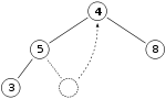
To add an element to a heap we must perform an up-heap operation (also known as bubble-up, percolate-up, sift-up, trickle-up, heapify-up, or cascade-up), by following this algorithm:
- Add the element to the bottom level of the heap.
- Compare the added element with its parent; if they are in the correct order, stop.
- If not, swap the element with its parent and return to the previous step.
The number of operations required depends only on the number of levels the new element must rise to satisfy the heap property, thus the insertion operation has a worst-case time complexity of O(log n) but an average-case complexity of O(1).
As an example of binary heap insertion, say we have a max-heap

and we want to add the number 15 to the heap. We first place the 15 in the position marked by the X. However, the heap property is violated since 15 > 8, so we need to swap the 15 and the 8. So, we have the heap looking as follows after the first swap:

However the heap property is still violated since 15 > 11, so we need to swap again:

which is a valid max-heap. There is no need to check the left child after this final step: at the start, the max-heap was valid, meaning 11 > 5; if 15 > 11, and 11 > 5, then 15 > 5, because of the transitive relation.
Extract
The procedure for deleting the root from the heap (effectively extracting the maximum element in a max-heap or the minimum element in a min-heap) and restoring the properties is called down-heap (also known as bubble-down, percolate-down, sift-down, trickle down, heapify-down, cascade-down, and extract-min/max).
- Replace the root of the heap with the last element on the last level.
- Compare the new root with its children; if they are in the correct order, stop.
- If not, swap the element with one of its children and return to the previous step. (Swap with its smaller child in a min-heap and its larger child in a max-heap.)
So, if we have the same max-heap as before

We remove the 11 and replace it with the 4.
Now the heap property is violated since 8 is greater than 4. In this case, swapping the two elements, 4 and 8, is enough to restore the heap property and we need not swap elements further:

The downward-moving node is swapped with the larger of its children in a max-heap (in a min-heap it would be swapped with its smaller child), until it satisfies the heap property in its new position. This functionality is achieved by the Max-Heapify function as defined below in pseudocode for an array-backed heap A of length heap_length[A]. Note that "A" is indexed starting at 1.
Max-Heapify (A, i):

    left ← 2*i // ← means "assignment"
    right ← 2*i + 1

    largest ← i


    if left ≤ heap_length[A] and A[left] > A[largest] then:

        largest ← left

    if right ≤ heap_length[A] and A[right] > A[largest] then:

        largest ← right


    if largest ≠ i then:

        swap A[i] and A[largest]
        Max-Heapify(A, largest)
For the above algorithm to correctly re-heapify the array, the node at index i and its two direct children must violate the heap property. If they do not, the algorithm will fall through with no change to the array. The down-heap operation (without the preceding swap) can also be used to modify the value of the root, even when an element is not being deleted. In the pseudocode above, what starts with // is a comment. Note that A is an array (or list) that starts being indexed from 1 up to length(A), according to the pseudocode.
In the worst case, the new root has to be swapped with its child on each level until it reaches the bottom level of the heap, meaning that the delete operation has a time complexity relative to the height of the tree, or O(log n).
Building a heap
Building a heap from an array of n input elements can be done by starting with an empty heap, then successively inserting each element. This approach, called Williams’ method after the inventor of binary heaps, is easily seen to run in O(n log n) time: it performs n insertions at O(log n) cost each.[lower-alpha 1]
However, Williams’ method is suboptimal. A faster method (due to Floyd[4]) starts by arbitrarily putting the elements on a binary tree, respecting the shape property (the tree could be represented by an array, see below). Then starting from the lowest level and moving upwards, sift the root of each subtree downward as in the deletion algorithm until the heap property is restored. More specifically if all the subtrees starting at some height have already been “heapified” (the bottommost level corresponding to ), the trees at height can be heapified by sending their root down along the path of maximum valued children when building a max-heap, or minimum valued children when building a min-heap. This process takes operations (swaps) per node. In this method most of the heapification takes place in the lower levels. Since the height of the heap is , the number of nodes at height is . Therefore, the cost of heapifying all subtrees is:


[lower-alpha 2] This uses the fact that the given infinite series converges.

The exact value of the above (the worst-case number of comparisons during the heap construction) is known to be equal to:
- ,[5]

where s2(n) is the sum of all digits of the binary representation of n and e2(n) is the exponent of 2 in the prime factorization of n.
The Build-Max-Heap function that follows, converts an array A which stores a complete binary tree with n nodes to a max-heap by repeatedly using Max-Heapify in a bottom up manner. It is based on the observation that the array elements indexed by floor(n/2) + 1, floor(n/2) + 2, ..., n are all leaves for the tree (assuming that indices start at 1), thus each is a one-element heap. Build-Max-Heap runs Max-Heapify on each of the remaining tree nodes.
Build-Max-Heap (A):

    heap_length[A] ← length[A]


    for each index i from floor(length[A]/2) downto 1 do:

        Max-Heapify(A, i)
Heap implementation
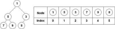
Heaps are commonly implemented with an array. Any binary tree can be stored in an array, but because a binary heap is always a complete binary tree, it can be stored compactly. No space is required for pointers; instead, the parent and children of each node can be found by arithmetic on array indices. These properties make this heap implementation a simple example of an implicit data structure or Ahnentafel list. Details depend on the root position, which in turn may depend on constraints of a programming language used for implementation, or programmer preference. Specifically, sometimes the root is placed at index 1, in order to simplify arithmetic.
Let n be the number of elements in the heap and i be an arbitrary valid index of the array storing the heap. If the tree root is at index 0, with valid indices 0 through n − 1, then each element a at index i has
- children at indices 2i + 1 and 2i + 2
- its parent at index floor((i − 1) ∕ 2).
Alternatively, if the tree root is at index 1, with valid indices 1 through n, then each element a at index i has
- children at indices 2i and 2i +1
- its parent at index floor(i ∕ 2).
This implementation is used in the heapsort algorithm, where it allows the space in the input array to be reused to store the heap (i.e. the algorithm is done in-place). The implementation is also useful for use as a Priority queue where use of a dynamic array allows insertion of an unbounded number of items.
The upheap/downheap operations can then be stated in terms of an array as follows: suppose that the heap property holds for the indices b, b+1, ..., e. The sift-down function extends the heap property to b−1, b, b+1, ..., e. Only index i = b−1 can violate the heap property. Let j be the index of the largest child of a[i] (for a max-heap, or the smallest child for a min-heap) within the range b, ..., e. (If no such index exists because 2i > e then the heap property holds for the newly extended range and nothing needs to be done.) By swapping the values a[i] and a[j] the heap property for position i is established. At this point, the only problem is that the heap property might not hold for index j. The sift-down function is applied tail-recursively to index j until the heap property is established for all elements.
The sift-down function is fast. In each step it only needs two comparisons and one swap. The index value where it is working doubles in each iteration, so that at most log2 e steps are required.
For big heaps and using virtual memory, storing elements in an array according to the above scheme is inefficient: (almost) every level is in a different page. B-heaps are binary heaps that keep subtrees in a single page, reducing the number of pages accessed by up to a factor of ten.[6]
The operation of merging two binary heaps takes Θ(n) for equal-sized heaps. The best you can do is (in case of array implementation) simply concatenating the two heap arrays and build a heap of the result.[7] A heap on n elements can be merged with a heap on k elements using O(log n log k) key comparisons, or, in case of a pointer-based implementation, in O(log n log k) time.[8] An algorithm for splitting a heap on n elements into two heaps on k and n-k elements, respectively, based on a new view of heaps as an ordered collections of subheaps was presented in.[9] The algorithm requires O(log n * log n) comparisons. The view also presents a new and conceptually simple algorithm for merging heaps. When merging is a common task, a different heap implementation is recommended, such as binomial heaps, which can be merged in O(log n).
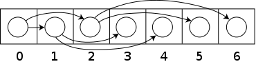
Additionally, a binary heap can be implemented with a traditional binary tree data structure, but there is an issue with finding the adjacent element on the last level on the binary heap when adding an element. This element can be determined algorithmically or by adding extra data to the nodes, called "threading" the tree—instead of merely storing references to the children, we store the inorder successor of the node as well.
It is possible to modify the heap structure to allow extraction of both the smallest and largest element in time.[10] To do this, the rows alternate between min heap and max heap. The algorithms are roughly the same, but, in each step, one must consider the alternating rows with alternating comparisons. The performance is roughly the same as a normal single direction heap. This idea can be generalised to a min-max-median heap.


Derivation of index equations
In an array-based heap, the children and parent of a node can be located via simple arithmetic on the node's index. This section derives the relevant equations for heaps with their root at index 0, with additional notes on heaps with their root at index 1.
To avoid confusion, we'll define the level of a node as its distance from the root, such that the root itself occupies level 0.
Child nodes
For a general node located at index (beginning from 0), we will first derive the index of its right child, .


Let node be located in level , and note that any level contains exactly nodes. Furthermore, there are exactly nodes contained in the layers up to and including layer (think of binary arithmetic; 0111...111 = 1000...000 - 1). Because the root is stored at 0, the th node will be stored at index . Putting these observations together yields the following expression for the index of the last node in layer l.


Let there be nodes after node in layer L, such that


Each of these nodes must have exactly 2 children, so there must be nodes separating 's right child from the end of its layer ( ).


As required.
Noting that the left child of any node is always 1 place before its right child, we get .

If the root is located at index 1 instead of 0, the last node in each level is instead at index . Using this throughout yields and for heaps with their root at 1.


Parent node
Every node is either the left or right child of its parent, so we know that either of the following is true.


Hence,

Now consider the expression .

If node is a left child, this gives the result immediately, however, it also gives the correct result if node is a right child. In this case, must be even, and hence must be odd.


Therefore, irrespective of whether a node is a left or right child, its parent can be found by the expression:

Related structures
Since the ordering of siblings in a heap is not specified by the heap property, a single node's two children can be freely interchanged unless doing so violates the shape property (compare with treap). Note, however, that in the common array-based heap, simply swapping the children might also necessitate moving the children's sub-tree nodes to retain the heap property.
The binary heap is a special case of the d-ary heap in which d = 2.
Summary of running times
In the following time complexities[11] O(f) is an asymptotic upper bound and Θ(f) is an asymptotically tight bound (see Big O notation). Function names assume a min-heap.
| Operation | Binary[11] | Leftist | Binomial[11] | Fibonacci[11][12] | Pairing[13] | Brodal[14][lower-alpha 3] | Rank-pairing[16] | Strict Fibonacci[17] | 2-3 heap |
|---|---|---|---|---|---|---|---|---|---|
| find-min | Θ(1) | Θ(1) | Θ(log n) | Θ(1) | Θ(1) | Θ(1) | Θ(1) | Θ(1) | ? |
| delete-min | Θ(log n) | Θ(log n) | Θ(log n) | O(log n)[lower-alpha 4] | O(log n)[lower-alpha 4] | O(log n) | O(log n)[lower-alpha 4] | O(log n) | O(log n)[lower-alpha 4] |
| insert | O(log n) | Θ(log n) | Θ(1)[lower-alpha 4] | Θ(1) | Θ(1) | Θ(1) | Θ(1) | Θ(1) | O(log n)[lower-alpha 4] |
| decrease-key | Θ(log n) | Θ(n) | Θ(log n) | Θ(1)[lower-alpha 4] | o(log n)[lower-alpha 4][lower-alpha 5] | Θ(1) | Θ(1)[lower-alpha 4] | Θ(1) | Θ(1) |
| merge | Θ(n) | Θ(log n) | O(log n)[lower-alpha 6] | Θ(1) | Θ(1) | Θ(1) | Θ(1) | Θ(1) | ? |
- ↑ In fact, this procedure can be shown to take Θ(n log n) time in the worst case, meaning that n log n is also an asymptotic lower bound on the complexity.[1]:167 In the average case (averaging over all permutations of n inputs), though, the method takes linear time.[4]
- ↑ This does not mean that sorting can be done in linear time since building a heap is only the first step of the heapsort algorithm.
- ↑ Brodal and Okasaki later describe a persistent variant with the same bounds except for decrease-key, which is not supported. Heaps with n elements can be constructed bottom-up in O(n).[15]
- 1 2 3 4 5 6 7 8 9 Amortized time.
- ↑ Lower bound of [18] upper bound of [19]
- ↑ n is the size of the larger heap.


See also
References
- 1 2 Cormen, Thomas H.; Leiserson, Charles E.; Rivest, Ronald L.; Stein, Clifford (2009) [1990]. Introduction to Algorithms (3rd ed.). MIT Press and McGraw-Hill. ISBN 0-262-03384-4.
- ↑ Williams, J. W. J. (1964), "Algorithm 232 - Heapsort", Communications of the ACM, 7 (6): 347–348, doi:10.1145/512274.512284
- ↑ eEL,CSA_Dept,IISc,Bangalore, "Binary Heaps", Data Structures and Algorithms
- 1 2 Hayward, Ryan; McDiarmid, Colin (1991). "Average Case Analysis of Heap Building by Repeated Insertion" (PDF). J. Algorithms. 12: 126–153. doi:10.1016/0196-6774(91)90027-v.
- ↑ Suchenek, Marek A. (2012), "Elementary Yet Precise Worst-Case Analysis of Floyd's Heap-Construction Program", Fundamenta Informaticae, IOS Press, 120 (1): 75–92, doi:10.3233/FI-2012-751 .
- ↑ Poul-Henning Kamp. "You're Doing It Wrong". ACM Queue. June 11, 2010.
- ↑ Chris L. Kuszmaul. "binary heap". Dictionary of Algorithms and Data Structures, Paul E. Black, ed., U.S. National Institute of Standards and Technology. 16 November 2009.
- ↑ J.-R. Sack and T. Strothotte "An Algorithm for Merging Heaps", Acta Informatica 22, 171-186 (1985).
- ↑ . J.-R. Sack and T. Strothotte "A characterization of heaps and its applications" Information and Computation Volume 86, Issue 1, May 1990, Pages 69–86.
- ↑ Atkinson, M.D.; J.-R. Sack; N. Santoro & T. Strothotte (1 October 1986). "Min-max heaps and generalized priority queues" (PDF). Programming techniques and Data structures. Comm. ACM, 29(10): 996–1000.
- 1 2 3 4 Cormen, Thomas H.; Leiserson, Charles E.; Rivest, Ronald L. (1990). Introduction to Algorithms (1st ed.). MIT Press and McGraw-Hill. ISBN 0-262-03141-8.
- ↑ Fredman, Michael Lawrence; Tarjan, Robert E. (July 1987). "Fibonacci heaps and their uses in improved network optimization algorithms" (PDF). Journal of the Association for Computing Machinery. 34 (3): 596&ndash, 615. doi:10.1145/28869.28874.
- ↑ Iacono, John (2000), "Improved upper bounds for pairing heaps", Proc. 7th Scandinavian Workshop on Algorithm Theory (PDF), Lecture Notes in Computer Science, 1851, Springer-Verlag, pp. 63–77, arXiv:1110.4428, doi:10.1007/3-540-44985-X_5, ISBN 3-540-67690-2
- ↑ Brodal, Gerth S. (1996), "Worst-Case Efficient Priority Queues" (PDF), Proc. 7th Annual ACM-SIAM Symposium on Discrete Algorithms, pp. 52–58
- ↑ Goodrich, Michael T.; Tamassia, Roberto (2004). "7.3.6. Bottom-Up Heap Construction". Data Structures and Algorithms in Java (3rd ed.). pp. 338&ndash, 341. ISBN 0-471-46983-1.
- ↑ Haeupler, Bernhard; Sen, Siddhartha; Tarjan, Robert E. (November 2011). "Rank-pairing heaps" (PDF). SIAM J. Computing: 1463–1485. doi:10.1137/100785351.
- ↑ Brodal, G. S. L.; Lagogiannis, G.; Tarjan, R. E. (2012). Strict Fibonacci heaps (PDF). Proceedings of the 44th symposium on Theory of Computing - STOC '12. p. 1177. doi:10.1145/2213977.2214082. ISBN 9781450312455.
- ↑ Fredman, Michael Lawrence (July 1999). "On the Efficiency of Pairing Heaps and Related Data Structures" (PDF). Journal of the Association for Computing Machinery. 46 (4): 473&ndash, 501. doi:10.1145/320211.320214.
- ↑ Pettie, Seth (2005). Towards a Final Analysis of Pairing Heaps (PDF). FOCS '05 Proceedings of the 46th Annual IEEE Symposium on Foundations of Computer Science. pp. 174&ndash, 183. CiteSeerX 10.1.1.549.471. doi:10.1109/SFCS.2005.75. ISBN 0-7695-2468-0.
External links
- Binary Heap Applet by Kubo Kovac
- Open Data Structures - Section 10.1 - BinaryHeap: An Implicit Binary Tree
- Implementation of binary max heap in C by Robin Thomas
- Implementation of binary min heap in C by Robin Thomas