Forms

z^2+c

Complex quadratic polynomial of the form :

$f_{c}(z)=z^{2}+c\,$

z^{n}+c\,

notation

"... typical notational convention is to parameterize critically preperiodic polynomials $z\to z^{2}+c$ by an angle $\theta$ of an external ray landing at the critical value rather than by c. In the event that more than one ray lands at the critical value, there may be multiple parameters referring to the same polynomial. As a simpler example, the polynomial:

$f_{1/6}=f_{i}$
for $\theta =1/4$ c= -0.228155493653962 +1.115142508039937 i
$f_{9/56}=f_{11/56}=f_{15/56}$

How to compute iteration

In Maxima CAS :

(%i28) z:zx+zy*%i;
(%o28) %i*zy+zx
(%i37) c:cx+cy*%i;
(%o37) %i*cy+cx
(%i38) realpart(z^2+c);
(%o38) -zy^2+zx^2+cx
(%i39) imagpart(z^2+c);
(%o39) 2*zx*zy+cy

Critical point

Critical orbits for various parabolic parameters on boundary of Main component of Mandelbrot set

A critical point of $f_{c}\,$ is a point $z_{cr}\,$ in the dynamical plane such that the derivative vanishes :

f_{c}'(z_{cr})=0.\,

Since

f_{c}'(z)={\frac {d}{dz}}f_{c}(z)=2z

implies

z_{cr}=0\,

One can see that :

the only (finite) critical point of $f_{c}\,$ is the point $z_{cr}=0\,$
critical point is the same for all c parameters

$z_{cr}$ is an initial point for Mandelbrot set iteration.^[2]

Dynamic plane

period 1 ( = fixed) points :^[3]

 $S_{1}(f_{c})={\frac {1}{2}}\pm {\frac {\sqrt {1-4c}}{2}}$

period 2 points :

 $S_{2}(f_{c})=-{\frac {1}{2}}\pm {\frac {\sqrt {-3-4c}}{2}}$

1/2

Julia set for parabolic parameter on the end fo 1/2 internal ray of main component of Mandelbrot set

First compute muliplier m of the fixed points using internal angle p/q and Maxima CAS:

${\frac {p}{q}}={\frac {1}{2}}$

(%i1) p:1$
(%i2) q:2$
(%i3) m:exp(2*%pi*%i*p/q);
(%o3)                                 - 1

Now compute parameter c of the function :

(%i1) GiveC(t,r):=
(
 [w,c],
 /* point of  unit circle   w:l(internalAngle,internalRadius); */
 w:r*%e^(%i*t*2*%pi),  /* point of circle */
 c:w/2-w*w/4, /* point on boundary of period 1 component of Mandelbrot set */
 float(rectform(c))    
)$

(%i3) c:GiveC(1/2,1);
(%o3) −0.75

Find fixed points z

(%i4) z1:z^2+c;
(%o4) z^2−0.75
(%i2) f:z^2+c;
(%o2)                              z^2  - 0.75
(%i3) d:diff(f,z,1);
(%o3)                                 2 z
(%i6) s:solve(z1=z);
(%o6)                              [z = 3/2, z = -1/2]
(%i7) s:map(rhs,s);
(%o7)                             [z = 3/2, z = -1/2]
(%i8) z:s[1];
(%o8)                                  3/2
(%i9) abs(float(rectform(ev(d))));
(%o9)                                 3.0
(%i10) z:s[2];
(%o10)                                - 1/2
(%i11) abs(float(rectform(ev(d))));
(%o11)                                1.0

So z=-1/2 is a parabolic fixed point.

z^2 + m*z

Complex quadratic polynomial of the form :

$f_{m}(z)=z^{2}+mz\,$

which has an indifferent fixed point^[4] with multiplier^[5]

$\lambda =m=e^{2\pi ti}\,$

at the origin^[6]^[7]

belongs to the class of the functions :

z^{n}+mz\,

How to compute iteration

In Maxima CAS :

(%i1) z:zx+zy*%i;
(%o1) %i*zy+zx
(%i2) m:mx+my*%i;
(%o2) %i*my+mx
(%i3) z1:z^2+m*z;
(%o3) (%i*zy+zx)^2+(%i*my+mx)*(%i*zy+zx)
(%i4) realpart(z1);
(%o4) -zy^2-my*zy+zx^2+mx*zx
(%i5) imagpart(z1);
(%o5) 2*zx*zy+mx*zy+my*zx

Critical point

A critical point of $f_{c}\,$ is a point $z_{cr}\,$ in the dynamical plane such that the derivative vanishes :

f_{m}'(z_{cr})=0.\,

Since

f_{m}'(z)={\frac {d}{dz}}f_{m}(z)=2z+m

implies

z_{cr}=-{\frac {m}{2}}\,

One can see that :

critical point is related with m value and have to be computed for every m parameters

$z_{cr}$ is an initial point for Mandelbrot set iteration.

Parameter plane lambda

parameter plane

period 1 components

(%i1) e1:z^2+m*z=z;
(%o1) z^2+m*z=z
(%i2) e2:2*z+m=w;
(%o2) 2*z+m=w
(%i3)  s:eliminate ([e1,e2], [z]);
(%o3) [-(m-w)*(w+m-2)]
(%i4) s:solve([s[1]], [m]);
(%o4) [m=2-w,m=w]

It means that there are 2 components of period 1 :

one with radius=1 and center=0 ( m=w )
second with radius=1 and center= -2 ( m=2-w)

How to compute boundary points of first component :

(%i1) m:exp(2*%pi*%i*p/q);
(%o1) %e^((2*%i*%pi*p)/q)
(%i2) realpart(m);
(%o2) cos((2*%pi*p)/q)
(%i3) imagpart(m);
(%o3) sin((2*%pi*p)/q)

Dynamic plane

1/1

Julia set for f(z) = z^2+z or f(z) = z^2 + 1/4 or f(z)= z-z^2

Domains for Fatou coordinate

Orbits of some points inside Julia set are shown ( white points)

First compute parameter of the function :

p:1$
q:1$
m:exp(2*%pi*%i*p/q);

The parameter is:

$m=e^{2\pi i}=1$

then the function is:

$f_{m}(z)=z^{2}+z$

it gives the same Julia set ( cauliflower ^[8] ) as function :

 $f_{c}(z)=z^{2}+{\frac {1}{4}}$

Compute fixed points :

(%i3) solve(z=z^2+z);
(%o3) [z=0]
(%i4) multiplicities;
(%o4) [2]

Find it's stability index = abs(multiplier) of the fixed point :

(%i1) f:z^2+z;
(%o1) z^2+z
(%i2) d:diff(f,z,1);
(%o2) 2*z+1
(%i7) z:0;
(%o7) 0
(%i8) abs(float(rectform(ev(d))));
(%o8) 1.0

Critical point :

$z_{cr}=-{\frac {m}{2}}=-{\frac {1}{2}}$

Iteration :

f(z):= z^2+z;

fn(n, z) :=
  if n=0 then z
  elseif n=1 then f(z)
  else f(fn(n-1, z));

1/2

First compute m = muliplier of the fixed points = parameter of the function f using internal angle p/q and Maxima CAS:

${\frac {p}{q}}={\frac {1}{2}}$

(%i1) p:1$
(%i2) q:2$
(%i3) m:exp(2*%pi*%i*p/q);
(%o3)                                 - 1

so function f is :

$f_{m}=z^{2}+mz=z^{2}-z$

How to compute iteration $z_{n+1}=f_{m}(z_{n})$ ?

(%i29) z1;
(%o29)                              z^2  - z
(%i30) z:zx+zy*%i;
(%o30)                            %i zy + zx
(%i32) realpart(ev(z1));
(%o32)                         - zy^2  + zx^2  - zx
(%i33) imagpart(ev(z1));
(%o33)                           2 zx zy - zy

Then find fixed points of f :

$z_{f}:\{z:f_{m}(z)=z\}$

(%i4) z1:z^2+m*z;
(%o4)                               z^2  - z
(%i5) zf:solve(z1=z);                                                  
(%o5)                           [z = 0, z = 2]
(%i6) multiplicities;
(%o6)                               [1, 1]

Stability of the fixed points :

(%i7) f:z1;
(%o7)                               z^2  - z
(%i8) d:diff(f,z,1);
(%o8)                               2 z - 1
(%i9) z:zf[1];   
(%o9)                                z = 0
(%i10) abs(ev(d));
(%o10)                         abs(2 z - 1) = 1
(%i11) z:zf[2];
(%o11)                               z = 2
(%i12) abs(ev(d));
(%o12)                         abs(2 z - 1) = 3
(%i13)

So fixed point :

z=0 is parabolic ( stability index = 1)
z=2 is repelling ( stability indexs = 3 , greater then 1 )

Find critical point $z_{cr}$ :

(%i14) zcr:solve(d=0);
(%o14)                              [z = 1/2]
(%i15) multiplicities;
(%o15)                                [1]

Attracting vectors

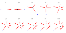
Because q=2, thus we examine 2-th iteration of f :

(%i16) z1;
(%o16)                              z^2  - z
(%i17) z2:z1^2-z1;
(%o17)                        (z^2  - z)^2  - z^2  + z
(%i18) taylor(z2,z,0,20);
taylor: z = 2 cannot be a variable.
 -- an error. To debug this try: debugmode(true);
(%i19) remvalue(z);
(%o19)                                [z]
(%i20) z;
(%o20)                                 z
(%i21) taylor(z2,z,0,20);
(%o21)/T/                    z - 2 z^3  + z^4  + . . .

Next term after z is a :

$-2z^{3}$

so here :

degree of above term is k=3
number of attracting directions ( and petals) is n= k-1 = 2 ( also n = e*q)
the parabolic degeneracy e = n/q = 1
cooefficient of above term a = -2

Attracing vectore satisfy :

$nav^{n}=-1$

so here :

$-4v^{2}=-1$

$v^{2}={\frac {1}{4}}$

One can solve it in Maxima CAS :

(%i22)  s:solve(z^2=1/4);
(%o22)                         [z = - 1/2, z =1/2]
(%i23) s:map(rhs,s);
(%o23)                             [-1/2, 1/2]
(%i24) carg_t(z):=
 block(
 [t],
 t:carg(z)/(2*%pi),  /* now in turns */
 if t<0 then t:t+1, /* map from (-1/2,1/2] to [0, 1) */
 return(t)
)$
(%i25)  s:map(carg_t,s);
(%o25)                              [1/2, 0]

So attracting vectors are :

$V_{a1}={\overrightarrow {v_{a1}0}}$ from $z=-{\frac {1}{2}}$ to the origin
$V_{a2}={\overrightarrow {v_{a2}0}}$ from $z={\frac {1}{2}}$ to the origin

Critical point z=1/2 lie on attracting vector $V_{a1}$ . Thus critical orbits tend straight to the origin under the iteration^[9]

Repelling vectors satisfy :

$nav^{n}=1$

so here :

$-4v^{2}=1$

$v^{2}=-{\frac {1}{4}}$

One can solve it in Maxima CAS :

(%i26) s:solve(z^2=-1/4);
(%o26)                        [z = - %i/2, z = %i/2]
(%i27) s:map(rhs,s);
(%o27)                            [- %i/2, %i/2 ]
(%i28) s:map(carg_t,s);
(%o28)                              [3/4, 1/4]

1/3

Critical orbit for f(z)=z^2 + mz where p over q=1 over 3

First compute parameter of the function :

/* Maxima CAS session */
(%i1) p:1;
      q:3;
      m:exp(2*%pi*%i*p/q);
(%o1) 1
(%o2) 3
(%o3) (sqrt(3)*%i)/2-1/2
(%i9) float(rectform(m));
(%o9) 0.86602540378444*%i-0.5

Then find fixed points :

/* Maxima CAS session */
(%i10) f:z^2+m*z;
(%o10) z^2+((sqrt(3)*%i)/2-1/2)*z
(%i11) z1:f;
(%o11) z^2+((sqrt(3)*%i)/2-1/2)*z
(%i12) solve(z1=z);
(%o12) [z=-(sqrt(3)*%i-3)/2,z=0]
(%i13) multiplicities;
(%o13) [1,1]

Compute multiplier of the fixed point :

(%i23) d:diff(f,z,1);
(%o23) 2*z+(sqrt(3)*%i)/2-1/2

Check stability of fixed points :

(%i12) s:solve(z1=z);
(%o12) [z=-(sqrt(3)*%i-3)/2,z=0]
(%i20) s:map(rectform,s);
(%o20) [3/2-(sqrt(3)*%i)/2,0]
(%i21) s:map('float,s);
(%o21) [1.5-0.86602540378444*%i,0.0]
(%i24) z:s[1];
(%o24) 1.5-0.86602540378444*%i;
(%i31) abs(float(rectform(ev(d))));
(%o31) 2.645751311064591

It means that fixed point z=1.5-0.86602540378444*%i is repelling.

Second point z=0 is parabolic :

(%i33) z:s[2];
(%o33) 0.0
(%i34) abs(float(rectform(ev(d))));
(%o34) 1.0

Find critical point :

(%i1) solve(2*z+(sqrt(3)*%i)/2-1/2);
(%o1) [z=-(sqrt(3)*%i-1)/4]
(%i2) s:solve(2*z+(sqrt(3)*%i)/2-1/2);
(%o2) [z=-(sqrt(3)*%i-1)/4]
(%i3) s:map(rhs,s);
(%o3) [-(sqrt(3)*%i-1)/4]
(%i4) s:map(rectform,s);
(%o4) [1/4-(sqrt(3)*%i)/4]
(%i5) s:map('float,s);
(%o5) [0.25-0.43301270189222*%i]
(%i6) abs(s[1]);
(%o6) 0.5

1/7

How to speed up computations ?

Approximate $f^{7}$ by :

$f_{a}^{7}(z)=(245.4962434402444i-234.5808769813032)*z^{8}+z$

How to compute $f_{a}^{7}$ :

(%i1) z:x+y*%i;
(%o1) %i*y+x
(%i2) z7:(245.4962434402444*%i-234.5808769813032)*z^8 + z;
(%o2) (245.4962434402444*%i-234.5808769813032)*(%i*y+x)^8+%i*y+x
(%i3) realpart(z7);
(%o3) -234.5808769813032*(y^8-28*x^2*y^6+70*x^4*y^4-28*x^6*y^2+x^8)-245.4962434402444*(-8*x*y^7+56*x^3*y^5-56*x^5*y^3+8*x^7*y)+x
(%i4) imagpart(z7);
(%o4) 245.4962434402444*(y^8-28*x^2*y^6+70*x^4*y^4-28*x^6*y^2+x^8)-234.5808769813032*(-8*x*y^7+56*x^3*y^5-56*x^5*y^3+8*x^7*y)+y

mz(1-z)

Description

at Mu-Ency ^[10]
at wikibook Pictures of Julia and Mandelbrot Sets

Critical points

critical points :

z = 1/2
z = ∞

Parameter plane

period 1 components

(%i1) e1:m*z*(1-z)=z;
(%o1) m*(1-z)*z=z
(%i2) d:diff(m*z*(1-z),z,1);
(%o2) m*(1-z)-m*z
(%i3) e2:d=w;
(%o3) m*(1-z)-m*z=w
(%i4) s:eliminate ([e1,e2], [z]);
(%o4) [m*(m-w)*(w+m-2)]
(%i5) s:solve([s[1]], [m]);
(%o5) [m=2-w,m=w,m=0]

It means that there are 2 period 1 components :

discs of radius 1 and centre in 0
disc of radius 1 and centre = 2

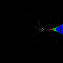
z(1-mz)

Dynamic plane

"Note that each member of the family of quadratic polynomials

 $\{g_{\lambda }:z\to z(1-\lambda z)\}_{\lambda \in C\setminus \{0\}}$

is parabolic since for each λ ∈ C \ {0}, the polynomial gλ has a parabolic fixed point 0 with miltiplicity 2 and the only finite critical point of $g_{\lambda }$ is given by

 ${\frac {1}{2\lambda }}$

which is contained in the basin of 0. The study of this family is too trivial since all its members are conjugate to

 $z\to z^{2}+{\frac {1}{4}}$

via Mobius transformations

 $h_{\lambda }(z)=-\lambda z+{\frac {1}{2}}$

and therefore all their Julia sets J(gλ) have the same Hausdorff dimension as

HD(J(z^2 +1/4)) ≈ 1.0812

"^[11]

z(1+ mz)

dynamic plane

z-z^2

Description ^[12]

First compute m = muliplier of the fixed points = parameter of the function f using internal angle p/q and Maxima CAS:

${\frac {p}{q}}={\frac {1}{2}}$

(%i1) p:1$
(%i2) q:2$
(%i3) m:exp(2*%pi*%i*p/q);
(%o3)                                 - 1

so function f is :

$f_{m}=z(1+mz)=z-z^{2}$

How to compute iteration $z_{n+1}=f_{m}(z_{n})$ ?

Find it using Maxima CAS :

(%i1) z:x+y*%i;
(%o1) %i*y+x
(%i2) z1:z-z^2;
(%o2) −(%i*y+x)^2+%i*y+x
(%i3) realpart(z1);
(%o3) y^2−x^2+x
(%i4) imagpart(z1);
(%o4) y−2*x*y

Then find fixed points of f :

$z_{f}:\{z:f_{m}(z)=z\}$

(%i6) remvalue(z);
(%o6) [z]
(%i7) zf:solve(z-z^2=z);
(%o7) [z=0]
(%i9) multiplicities;
(%o9) [2]

Stability of the fixed points :

(%i11) f:z-z^2;
(%o11) z−z^2
(%i12) d:diff(f,z,1);
(%o12) 1−2*z
(%i13) zf:solve(z-z^2=z);
(%o13) [z=0]
(%i14) z:zf[1];
(%o14) z=0
(%i15) abs(ev(d));
(%o15) abs(2*z−1)=1

It means that fixed point z=0 is a parabolic point ( stability indeks = 1 ).

Find critical point $z_{cr}$ :

(%i16) zcr:solve(d=0);
(%o16) [z=1/2]

This article is issued from Wikibooks. The text is licensed under Creative Commons - Attribution - Sharealike. Additional terms may apply for the media files.

[1] wikipedia : Complex quadratic polynomial - definition

[2] Java program by Dieter Röß showing result of changing initial point of Mandelbrot iterations

[3] Algebraic Geometry of Discrete Dynamics The case of one variable V.Dolotin and A.Morozov

[4] wikipedia : fixed point

[5] wikipedia : multiplier

[6] wikipedia : origin

[7] Michael Yampolsky, Saeed Zakeri : Mating Siegel quadratic polynomials.

[8] s of Cauliflower_Julia_set

[9] Mark McClure in stackexchange questions : what-is-the-shape-of-parabolic-critical-orbit

[10] t Mu-Ency

[11] REAL ANALYTICITY OF HAUSDORFF DIMENSION OF DISCONNECTED JULIA SETS OF CUBIC PARABOLIC POLYNOMIALS Hasina Akter

[12] S Lapan : On the existence of attracting domains for maps tangent to the identity. Ph.D. Thesis, University of Michigan

Forms

z^2+c

notation

How to compute iteration

Critical point

Dynamic plane

1/2

z^2 + m*z

How to compute iteration

Critical point

parameter plane

period 1 components

Dynamic plane

1/1

1/2

1/3

1/7

m*z*(1-z)

Critical points

Parameter plane

period 1 components

z(1-mz)

Dynamic plane

z(1+ mz)

dynamic plane

z-z^2

References

mz(1-z)