Projection (linear algebra)
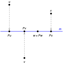
In linear algebra and functional analysis, a projection is a linear transformation from a vector space to itself such that . That is, whenever is applied twice to any value, it gives the same result as if it were applied once (idempotent). It leaves its image unchanged.[1] Though abstract, this definition of "projection" formalizes and generalizes the idea of graphical projection. One can also consider the effect of a projection on a geometrical object by examining the effect of the projection on points in the object.


Definitions
A projection on a vector space is a linear operator such that .


When has an inner product and is complete (i.e. when is a Hilbert space) the concept of orthogonality can be used. A projection on a Hilbert space is called an orthogonal projection if it satisfies for all . A projection on a Hilbert space that is not orthogonal is called an oblique projection.


Projection matrix
- In the finite-dimensional case, a square matrix is called a projection matrix if it is equal to its square, i.e. if .[2]:p. 38
- A square matrix is called an orthogonal projection matrix if for a real matrix, and respectively for a complex matrix, where denotes the transpose of and denotes the Hermitian transpose of .[2]:p. 223
- A projection matrix that is not an orthogonal projection matrix is called an oblique projection matrix.


The eigenvalues of a projection matrix must be 0 or 1.
Examples
Orthogonal projection
For example, the function which maps the point in three-dimensional space to the point is an orthogonal projection onto the x–y plane. This function is represented by the matrix


The action of this matrix on an arbitrary vector is

To see that is indeed a projection, i.e., , we compute

- .

Observing that shows that the projection is an orthogonal projection.

Oblique projection
A simple example of a non-orthogonal (oblique) projection (for definition see below) is

Via matrix multiplication, one sees that

proving that is indeed a projection.
The projection is orthogonal if and only if because only then .

Properties and classification
Idempotence
By definition, a projection is idempotent (i.e. ).
Complementarity of range and kernel
Let be a finite dimensional vector space and be a projection on . Suppose the subspaces and are the range and kernel of respectively. Then has the following properties:


- is the identity operator on
- .
- We have a direct sum . Every vector may be decomposed uniquely as with and , and where .


The range and kernel of a projection are complementary, as are and . The operator is also a projection as the range and kernel of become the kernel and range of and vice versa. We say is a projection along onto (kernel/range) and is a projection along onto .


Spectrum
In infinite dimensional vector spaces, the spectrum of a projection is contained in as


Only 0 or 1 can be an eigenvalue of a projection, implying that is always a positive semi-definite matrix. The corresponding eigenspaces are (respectively) the kernel and range of the projection. Decomposition of a vector space into direct sums is not unique in general. Therefore, given a subspace , there may be many projections whose range (or kernel) is .
If a projection is nontrivial it has minimal polynomial , which factors into distinct roots, and thus is diagonalizable.

Product of projections
The product of projections is not in general a projection, even if they are orthogonal. If two projections commute then their product is a projection, but the converse if false: the product of two non-commuting projections may be a projection .
If two orthogonal projections commute then their product is an orthogonal projection. If the product of two orthogonal projections is an orthogonal projection, then the two orthogonal projections commute (more generally: two self-adjoint endomorphisms commute if and only if their product is self-adjoint).
Orthogonal projections
When the vector space has an inner product and is complete (is a Hilbert space) the concept of orthogonality can be used. An orthogonal projection is a projection for which the range and the null space are orthogonal subspaces. Thus, for every and in , . Equivalently:


- .

A projection is orthogonal if and only if it is self-adjoint. Using the self-adjoint and idempotent properties of , for any and in we have , , and


where is the inner product associated with . Therefore, and are orthogonal projections.[3] The other direction, namely that if is orthogonal then it is self-adjoint, follows from


for every and in ; thus .

Proof of existence Let be a complete metric space with an inner product, and let be a closed linear subspace of (and hence complete as well).
For every the following set of non-negative norms has an infimum, and due to the completeness of it is a minimum. We define as the point in where this minimum is obtained.
Obviously is in . It remains to show that satisfies and that it is linear.
Let us define . For every non-zero in , the following holds:
By defining we see that unless vanishes. Since was chosen as the minimum of the abovementioned set, it follows that indeed vanishes. In particular, (for ): .
Linearity follows from the vanishing of for every :
By taking the difference between the equations we have
But since we may choose (as it is itself in ) it follows that . Similarly we have for every scalar .


Properties and special cases
An orthogonal projection is a bounded operator. This is because for every in the vector space we have, by Cauchy–Schwarz inequality:

Thus .

For finite dimensional complex or real vector spaces, the standard inner product can be substituted for .
Formulas
A simple case occurs when the orthogonal projection is onto a line. If is a unit vector on the line, then the projection is given by the outer product


(If is complex-valued, the transpose in the above equation is replaced by a Hermitian transpose). This operator leaves u invariant, and it annihilates all vectors orthogonal to , proving that it is indeed the orthogonal projection onto the line containing u.[4] A simple way to see this is to consider an arbitrary vector as the sum of a component on the line (i.e. the projected vector we seek) and another perpendicular to it, . Applying projection, we get


by the properties of the dot product of parallel and perpendicular vectors.
This formula can be generalized to orthogonal projections on a subspace of arbitrary dimension. Let be an orthonormal basis of the subspace , and let denote the matrix whose columns are , i.e . Then the projection is given by:[5]


which can be rewritten as

The matrix is the partial isometry that vanishes on the orthogonal complement of and is the isometry that embeds into the underlying vector space. The range of is therefore the final space of . It is also clear that is the identity operator on .


The orthonormality condition can also be dropped. If is a (not necessarily orthonormal) basis, and is the matrix with these vectors as columns, then the projection is:[6][7]

The matrix still embeds into the underlying vector space but is no longer an isometry in general. The matrix is a "normalizing factor" that recovers the norm. For example, the rank-1 operator is not a projection if After dividing by we obtain the projection onto the subspace spanned by .


In the general case, we can have an arbitrary positive definite matrix defining an inner product , and the projection is given by . Then


When the range space of the projection is generated by a frame (i.e. the number of generators is greater than its dimension), the formula for the projection takes the form: . Here stands for the Moore–Penrose pseudoinverse. This is just one of many ways to construct the projection operator.


If is a non-singular matrix and (i.e., is the null space matrix of ),[8] the following holds:


If the orthogonal condition is enhanced to with non-singular, the following holds:


All these formulas also hold for complex inner product spaces, provided that the conjugate transpose is used instead of the transpose. Further details on sums of projectors can be found in Banerjee and Roy (2014).[9] Also see Banerjee (2004)[10] for application of sums of projectors in basic spherical trigonometry.
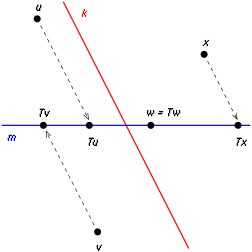
Oblique projections
The term oblique projections is sometimes used to refer to non-orthogonal projections. These projections are also used to represent spatial figures in two-dimensional drawings (see oblique projection), though not as frequently as orthogonal projections. Whereas calculating the fitted value of an ordinary least squares regression requires an orthogonal projection, calculating the fitted value of an instrumental variables regression requires an oblique projection.
Projections are defined by their null space and the basis vectors used to characterize their range (which is the complement of the null space). When these basis vectors are orthogonal to the null space, then the projection is an orthogonal projection. When these basis vectors are not orthogonal to the null space, the projection is an oblique projection. Let the vectors form a basis for the range of the projection, and assemble these vectors in the matrix . The range and the null space are complementary spaces, so the null space has dimension . It follows that the orthogonal complement of the null space has dimension . Let form a basis for the orthogonal complement of the null space of the projection, and assemble these vectors in the matrix . Then the projection is defined by


This expression generalizes the formula for orthogonal projections given above.[11][12]
Finding projection with an inner product
Let be a vector space (in this case a plane) spanned by orthogonal vectors . Let be a vector. One can define a projection of onto as


where the 's and 's imply Einstein sum notation. The vector can be written as an orthogonal sum such that . is sometimes denoted as . There is a theorem in Linear Algebra that states that this is the shortest distance from to and is commonly used in areas such as machine learning.


Canonical forms
Any projection on a vector space of dimension over a field is a diagonalizable matrix, since its minimal polynomial divides , which splits into distinct linear factors. Thus there exists a basis in which has the form


where is the rank of . Here is the identity matrix of size , and is the zero matrix of size . If the vector space is complex and equipped with an inner product, then there is an orthonormal basis in which the matrix of P is[13]


- .

where . The integers and the real numbers are uniquely determined. Note that . The factor corresponds to the maximal invariant subspace on which acts as an orthogonal projection (so that P itself is orthogonal if and only if ) and the -blocks correspond to the oblique components.


Projections on normed vector spaces
When the underlying vector space is a (not necessarily finite-dimensional) normed vector space, analytic questions, irrelevant in the finite-dimensional case, need to be considered. Assume now is a Banach space.

Many of the algebraic results discussed above survive the passage to this context. A given direct sum decomposition of into complementary subspaces still specifies a projection, and vice versa. If is the direct sum , then the operator defined by is still a projection with range and kernel . It is also clear that . Conversely, if is projection on , i.e. , then it is easily verified that . In other words, is also a projection. The relation implies and is the direct sum .


However, in contrast to the finite-dimensional case, projections need not be continuous in general. If a subspace of is not closed in the norm topology, then projection onto is not continuous. In other words, the range of a continuous projection must be a closed subspace. Furthermore, the kernel of a continuous projection (in fact, a continuous linear operator in general) is closed. Thus a continuous projection gives a decomposition of into two complementary closed subspaces: .

The converse holds also, with an additional assumption. Suppose is a closed subspace of . If there exists a closed subspace such that X = U ⊕ V, then the projection with range and kernel is continuous. This follows from the closed graph theorem. Suppose xn → x and Pxn → y. One needs to show that . Since is closed and {Pxn} ⊂ U, y lies in , i.e. Py = y. Also, xn − Pxn = (I − P)xn → x − y. Because is closed and {(I − P)xn} ⊂ V, we have , i.e. , which proves the claim.


The above argument makes use of the assumption that both and are closed. In general, given a closed subspace , there need not exist a complementary closed subspace , although for Hilbert spaces this can always be done by taking the orthogonal complement. For Banach spaces, a one-dimensional subspace always has a closed complementary subspace. This is an immediate consequence of Hahn–Banach theorem. Let be the linear span of . By Hahn–Banach, there exists a bounded linear functional such that φ(u) = 1. The operator satisfies , i.e. it is a projection. Boundedness of implies continuity of and therefore is a closed complementary subspace of .


Applications and further considerations
Projections (orthogonal and otherwise) play a major role in algorithms for certain linear algebra problems:
- QR decomposition (see Householder transformation and Gram–Schmidt decomposition);
- Singular value decomposition
- Reduction to Hessenberg form (the first step in many eigenvalue algorithms)
- Linear regression
- Projective elements of matrix algebras are used in the construction of certain K-groups in Operator K-theory
As stated above, projections are a special case of idempotents. Analytically, orthogonal projections are non-commutative generalizations of characteristic functions. Idempotents are used in classifying, for instance, semisimple algebras, while measure theory begins with considering characteristic functions of measurable sets. Therefore, as one can imagine, projections are very often encountered in the context operator algebras. In particular, a von Neumann algebra is generated by its complete lattice of projections.
Generalizations
More generally, given a map between normed vector spaces one can analogously ask for this map to be an isometry on the orthogonal complement of the kernel: that be an isometry (compare Partial isometry); in particular it must be onto. The case of an orthogonal projection is when W is a subspace of V. In Riemannian geometry, this is used in the definition of a Riemannian submersion.


See also
- Centering matrix, which is an example of a projection matrix.
- Orthogonalization
- Invariant subspace
- Properties of trace
- Dykstra's projection algorithm to compute the projection onto an intersection of sets
Notes
- Meyer, pp 386+387
- Horn, Roger A.; Johnson, Charles R. (2013). Matrix Analysis, second edition. Cambridge University Press. ISBN 9780521839402.
- Meyer, p. 433
- Meyer, p. 431
- Meyer, equation (5.13.4)
- Banerjee, Sudipto; Roy, Anindya (2014), Linear Algebra and Matrix Analysis for Statistics, Texts in Statistical Science (1st ed.), Chapman and Hall/CRC, ISBN 978-1420095388
- Meyer, equation (5.13.3)
- See also Linear least squares (mathematics) § Properties of the least-squares estimators.
- Banerjee, Sudipto; Roy, Anindya (2014), Linear Algebra and Matrix Analysis for Statistics, Texts in Statistical Science (1st ed.), Chapman and Hall/CRC, ISBN 978-1420095388
- Banerjee, Sudipto (2004), "Revisiting Spherical Trigonometry with Orthogonal Projectors", The College Mathematics Journal, 35: 375–381, doi:10.1080/07468342.2004.11922099
- Banerjee, Sudipto; Roy, Anindya (2014), Linear Algebra and Matrix Analysis for Statistics, Texts in Statistical Science (1st ed.), Chapman and Hall/CRC, ISBN 978-1420095388
- Meyer, equation (7.10.39)
- Doković, D. Ž. (August 1991). "Unitary similarity of projectors". Aequationes Mathematicae. 42 (1): 220–224. doi:10.1007/BF01818492.
References
- Banerjee, Sudipto; Roy, Anindya (2014), Linear Algebra and Matrix Analysis for Statistics, Texts in Statistical Science (1st ed.), Chapman and Hall/CRC, ISBN 978-1420095388
- Dunford, N.; Schwartz, J. T. (1958). Linear Operators, Part I: General Theory. Interscience.
- Meyer, Carl D. (2000). Matrix Analysis and Applied Linear Algebra. Society for Industrial and Applied Mathematics. ISBN 978-0-89871-454-8.
External links
- MIT Linear Algebra Lecture on Projection Matrices on YouTube, from MIT OpenCourseWare
- Linear Algebra 15d: The Projection Transformation on YouTube, by Pavel Grinfeld.
- Planar Geometric Projections Tutorial – a simple-to-follow tutorial explaining the different types of planar geometric projections.
| Basic concepts |
|  |
|---|---|---|
| Vector algebra |
| |
| Multilinear algebra |
| |
| Matrices |
| |
| Algebraic constructions |
| |
| Numerical |
| |
| ||