Likelihood function

Let ${\displaystyle X}$ be a discrete random variable with probability mass function ${\displaystyle p}$ depending on a parameter ${\displaystyle \theta }$. Then the function

${\displaystyle {\mathcal {L}}(\theta \mid x)=p_{\theta }(x)=P_{\theta }(X=x),}$

considered as a function of ${\displaystyle \theta }$, is the likelihood function, given the outcome ${\displaystyle x}$ of the random variable ${\displaystyle X}$. Sometimes the probability of "the value ${\displaystyle x}$ of ${\displaystyle X}$ for the parameter value ${\displaystyle \theta }$ " is written as P(X = x | θ) or P(X = x; θ). ${\displaystyle {\mathcal {L}}(\theta \mid x)}$ should not be confused with ${\displaystyle p(\theta \mid x)}$; the likelihood is equal to the probability that a particular outcome ${\displaystyle x}$ is observed when the true value of the parameter is ${\displaystyle \theta }$, and hence it is equal to a probability density over the outcome ${\displaystyle x}$, not over the parameter ${\displaystyle \theta }$.

Figure 1.  The likelihood function (${\displaystyle p_{\text{H}}^{2}}$) for the probability of a coin landing heads-up (without prior knowledge of the coin's fairness), given that we have observed HH.

Figure 2.  The likelihood function (${\displaystyle p_{\text{H}}^{2}(1-p_{\text{H}})}$) for the probability of a coin landing heads-up (without prior knowledge of the coin's fairness), given that we have observed HHT.

Consider a simple statistical model of a coin flip: a single parameter ${\displaystyle p_{\text{H}}}$ that expresses the "fairness" of the coin. The parameter is the probability that a coin lands heads up ("H") when tossed. ${\displaystyle p_{\text{H}}}$ can take on any value within the range 0.0 to 1.0. For a perfectly fair coin, ${\displaystyle p_{\text{H}}=0.5}$.

Imagine flipping a fair coin twice, and observing the following data: two heads in two tosses ("HH"). Assuming that each successive coin flip is i.i.d., then the probability of observing HH is

${\displaystyle P({\text{HH}}\mid p_{\text{H}}=0.5)=0.5^{2}=0.25.}$

Hence, given the observed data HH, the likelihood that the model parameter ${\displaystyle p_{\text{H}}}$ equals 0.5 is 0.25. Mathematically, this is written as

${\displaystyle {\mathcal {L}}(p_{\text{H}}=0.5\mid {\text{HH}})=0.25.}$

This is not the same as saying that the probability that ${\displaystyle p_{\text{H}}=0.5}$, given the observation HH, is 0.25. (For that, we could apply Bayes' theorem, which implies that the posterior probability is proportional to the likelihood times the prior probability.)

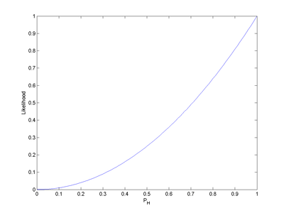
Suppose that the coin is not a fair coin, but instead it has ${\displaystyle p_{\text{H}}=0.3}$. Then the probability of getting two heads is

${\displaystyle P({\text{HH}}\mid p_{\text{H}}=0.3)=0.3^{2}=0.09.}$

Hence

${\displaystyle {\mathcal {L}}(p_{\text{H}}=0.3\mid {\text{HH}})=0.09.}$

More generally, for each value of ${\displaystyle p_{\text{H}}}$, we can calculate the corresponding likelihood. The result of such calculations is displayed in Figure 1.

In Figure 1, the integral of the likelihood over the interval [0, 1] is 1/3. That illustrates an important aspect of likelihoods: likelihoods do not have to integrate (or sum) to 1, unlike probabilities.

Let ${\displaystyle X}$ be a random variable following an absolutely continuous probability distribution with density function ${\displaystyle f}$ depending on a parameter ${\displaystyle \theta }$. Then the function

${\displaystyle {\mathcal {L}}(\theta \mid x)=f_{\theta }(x)=p(X=x\mid \theta ),\,}$

considered as a function of ${\displaystyle \theta }$, is the likelihood function (of ${\displaystyle \theta }$, given the outcome ${\displaystyle x}$ of ${\displaystyle X}$). Sometimes the density function for "the value ${\displaystyle x}$ of ${\displaystyle X}$ for the parameter value ${\displaystyle \theta }$ " is written as ${\displaystyle f(x\mid \theta )}$. ${\displaystyle {\mathcal {L}}(\theta \mid x)}$ should not be confused with ${\displaystyle p(\theta \mid x)}$; the likelihood is equal to the probability density at a particular outcome ${\displaystyle x}$ when the true value of the parameter is ${\displaystyle \theta }$, and hence it is equal to a probability density over the outcome ${\displaystyle x}$, not over the parameter ${\displaystyle \theta }$.

In measure-theoretic probability theory, the density function is defined as the Radon–Nikodym derivative of the probability distribution relative to a common dominating measure.[7] The likelihood function is that density interpreted as a function of the parameter (possibly a vector), rather than the possible outcomes.[8] This provides a likelihood function for any statistical model with all distributions, whether discrete, absolutely continuous, a mixture or something else. (Likelihoods will be comparable, e.g. for parameter estimation, only if they are Radon–Nikodym derivatives with respect to the same dominating measure.)

The discussion above of likelihood with discrete probabilities is a special case of this using the counting measure, which makes the probability of any single outcome equal to the probability density for that outcome.

Given no event (no data), the probability and thus likelihood is 1; any non-trivial event will have a lower likelihood.

Among many applications, we consider here one of broad theoretical and practical importance. Given a parameterized family of probability density functions (or probability mass functions in the case of discrete distributions)

${\displaystyle x\mapsto f(x\mid \theta ),\!}$

where ${\displaystyle \theta }$ is the parameter, the likelihood function is

${\displaystyle \theta \mapsto f(x\mid \theta ),\!}$

written

${\displaystyle {\mathcal {L}}(\theta \mid x)=f(x\mid \theta ),\!}$

where ${\displaystyle x}$ is the observed outcome of an experiment. In other words, when ${\displaystyle f(x|\theta )}$ is viewed as a function of ${\displaystyle x}$ with ${\displaystyle \theta }$ fixed, it is a probability density function, and when viewed as a function of ${\displaystyle \theta }$ with ${\displaystyle x}$ fixed, it is a likelihood function.

This is not the same as the probability that those parameters are the right ones, given the observed sample. Attempting to interpret the likelihood of a hypothesis given observed evidence as the probability of the hypothesis is a common error, with potentially disastrous consequences. See prosecutor's fallacy for an example of this.

From a geometric standpoint, if we consider ${\displaystyle f(x|\theta )}$ as a function of two variables then the family of probability distributions can be viewed as a family of curves parallel to the ${\displaystyle x}$-axis, while the family of likelihood functions is the orthogonal curves parallel to the ${\displaystyle \theta }$-axis.

The use of the probability density in specifying the likelihood function above is justified as follows. Given an observation ${\displaystyle x_{j}}$, the likelihood for the interval ${\displaystyle [x_{j},x_{j}+h]}$, where ${\displaystyle h>0}$ is a constant, is given by ${\displaystyle {\mathcal {L}}(\theta \mid x\in [x_{j},x_{j}+h])}$. Observe that

${\displaystyle \operatorname {argmax} _{\theta }{\mathcal {L}}(\theta \mid x\in [x_{j},x_{j}+h])=\operatorname {argmax} _{\theta }{\frac {1}{h}}{\mathcal {L}}(\theta \mid x\in [x_{j},x_{j}+h])}$,

since ${\displaystyle h}$ is positive and constant. Because

${\displaystyle \operatorname {argmax} _{\theta }{\frac {1}{h}}{\mathcal {L}}(\theta \mid x\in [x_{j},x_{j}+h])=\operatorname {argmax} _{\theta }{\frac {1}{h}}\Pr(x_{j}\leq x\leq x_{j}+h\mid \theta )=\operatorname {argmax} _{\theta }{\frac {1}{h}}\int _{x_{j}}^{x_{j}+h}f(x\mid \theta )\,dx,}$

where ${\displaystyle f(x\mid \theta )}$ is the probability density function, it follows that

${\displaystyle \operatorname {argmax} _{\theta }{\mathcal {L}}(\theta \mid x\in [x_{j},x_{j}+h])=\operatorname {argmax} _{\theta }{\frac {1}{h}}\int _{x_{j}}^{x_{j}+h}f(x\mid \theta )\,dx}$.

The first fundamental theorem of calculus and the l'Hôpital's rule together provide that

${\displaystyle {\begin{aligned}&\lim _{h\to 0^{+}}{\frac {1}{h}}\int _{x_{j}}^{x_{j}+h}f(x\mid \theta )\,dx=\lim _{h\to 0^{+}}{\frac {{\frac {d}{dh}}\int _{x_{j}}^{x_{j}+h}f(x\mid \theta )\,dx}{\frac {dh}{dh}}}\\[4pt]={}&\lim _{h\to 0^{+}}{\frac {f(x_{j}+h\mid \theta )}{1}}=f(x_{j}\mid \theta ).\end{aligned}}}$

Then

${\displaystyle {\begin{aligned}&\operatorname {argmax} _{\theta }{\mathcal {L}}(\theta \mid x_{j})=\operatorname {argmax} _{\theta }\left[\lim _{h\to 0^{+}}{\mathcal {L}}(\theta \mid x\in [x_{j},x_{j}+h])\right]\\[4pt]={}&\operatorname {argmax} _{\theta }\left[\lim _{h\to 0^{+}}{\frac {1}{h}}\int _{x_{j}}^{x_{j}+h}f(x\mid \theta )\,dx\right]=\operatorname {argmax} _{\theta }f(x_{j}\mid \theta ).\end{aligned}}}$

Therefore,

${\displaystyle \operatorname {argmax} _{\theta }{\mathcal {L}}(\theta \mid x_{j})=\operatorname {argmax} _{\theta }f(x_{j}\mid \theta ),\!}$

and so maximizing the probability density at ${\displaystyle x_{j}}$ amounts to maximizing the likelihood of the specific observation ${\displaystyle x_{j}}$.

The above can be extended in a simple way to allow consideration of distributions which contain both discrete and continuous components. Suppose that the distribution consists of a number of discrete probability masses ${\displaystyle p_{k}\theta }$ and a density ${\displaystyle f(x|\theta )}$, where the sum of all the ${\displaystyle p}$'s added to the integral of ${\displaystyle f}$ is always one. Assuming that it is possible to distinguish an observation corresponding to one of the discrete probability masses from one which corresponds to the density component, the likelihood function for an observation from the continuous component can be dealt with in the manner shown above. For an observation from the discrete component, the likelihood function for an observation from the discrete component is simply

${\displaystyle {\mathcal {L}}(\theta \mid x)=p_{k}(\theta ),\!}$

where ${\displaystyle k}$ is the index of the discrete probability mass corresponding to observation ${\displaystyle x}$, because maximizing the probability mass (or probability) at ${\displaystyle x}$ amounts to maximizing the likelihood of the specific observation.

The fact that the likelihood function can be defined in a way that includes contributions that are not commensurate (the density and the probability mass) arises from the way in which the likelihood function is defined up to a constant of proportionality, where this "constant" can change with the observation ${\displaystyle x}$, but not with the parameter ${\displaystyle \theta }$.

In the context of parameter estimation, the likelihood function is usually assumed to obey certain conditions, known as regularity conditions. These conditions are assumed in various proofs involving likelihood functions, and need to be verified in each particular application. For maximum likelihood estimation, the existence of a global maximum of the likelihood function is of the utmost importance. By the extreme value theorem, a continuous likelihood function on a compact parameter space suffices for the existence of a maximum likelihood estimator.[9] While the continuity assumption is usually met, the compactness assumption about the parameter space is often not, as the bounds of the true parameter values are unknown. In that case, concavity of the likelihood function plays a key role.

More specifically, if the likelihood function is twice continuously differentiable on the k-dimensional parameter space ${\displaystyle \Theta }$ assumed to be an open connected subset of ${\displaystyle \mathbb {R} ^{k}}$, there exists a unique maximum ${\displaystyle {\hat {\theta }}\in \Theta }$ if

${\displaystyle \mathbf {H} (\theta )=\left\{{\frac {\partial ^{2}L}{\partial \theta _{i}\partial \theta _{j}}}\right\}}$ is negative definite at every ${\displaystyle \theta \in \Theta }$ for which gradient ${\displaystyle \nabla L=\left\{\partial L/\partial \theta _{i}\right\}}$ vanishes, and

${\displaystyle \lim _{\theta \to \partial \Theta }L(\theta )=0}$, i.e. the likelihood function approaches a constant on the boundary of the parameter space, which may include the points at infinity if ${\displaystyle \Theta }$ is unbounded.

Mäkeläinen et al. prove this result using Morse theory while informally appealing to a mountain pass property.[10] Mascarenhas restates their proof using the mountain pass theorem.[11]

In the proofs of consistency and asymptotic normality of the maximum likelihood estimator, additional assumptions are made about the probability densities that form the basis of a particular likelihood function. These conditions were first established by Chanda.[12] In particular, for almost all ${\displaystyle x}$, and for all ${\displaystyle \theta \in \Theta }$,

${\displaystyle {\frac {\partial \log f}{\partial \theta _{r}}}\,,\quad {\frac {\partial ^{2}\log f}{\partial \theta _{r}\partial \theta _{s}}}\,,\quad {\frac {\partial ^{3}\log f}{\partial \theta _{r}\partial \theta _{s}\partial \theta _{t}}}}$

exist for all ${\displaystyle r,s,t=1,2,\ldots ,k}$ in order to ensure the existence of a Taylor expansion. Second, for almost all ${\displaystyle x}$ and for every ${\displaystyle \theta \in \Theta }$ it must be that

${\displaystyle \left|{\frac {\partial f}{\partial \theta _{r}}}\right|<F_{r}(x)\,,\quad \left|{\frac {\partial ^{2}f}{\partial \theta _{r}\partial \theta _{s}}}\right|<F_{rs}(x)\,,\quad \left|{\frac {\partial ^{3}f}{\partial \theta _{r}\partial \theta _{s}\partial \theta _{t}}}\right|<H_{rst}(x)}$

where ${\displaystyle H}$ is such that ${\displaystyle \int _{-\infty }^{\infty }H_{rst}(z)\mathrm {d} z\leq M<\infty }$. This boundedness of the derivatives is needed to allow for differentiation under the integral sign. And lastly, it is assumed that the information matrix,

${\displaystyle \mathbf {I} (\theta )=\int _{-\infty }^{\infty }{\frac {\partial \log f}{\partial \theta _{r}}}{\frac {\partial \log f}{\partial \theta _{s}}}f\mathrm {d} z}$

is positive definite and ${\displaystyle \left|\mathbf {I} (\theta )\right|}$ is finite. This ensures that the score has a finite variance.[13]

The above conditions are sufficient, but not necessary. That is, a model that does not meet these regularity conditions may or may not have a maximum likelihood estimator of the properties mentioned above. Further, in case of non-independently or non-identically distributed observations additional properties may need to be assumed.

A likelihood ratio is the ratio of any two specified likelihoods, frequently written as:

${\displaystyle \Lambda (\theta _{1}:\theta _{2}\mid x)={\frac {{\mathcal {L}}(\theta _{1}\mid x)}{{\mathcal {L}}(\theta _{2}\mid x)}}}$

The likelihood ratio is central to likelihoodist statistics: the law of likelihood states that degree to which data (considered as evidence) supports one parameter value versus another is measured by the likelihood ratio.

In frequentist inference, the likelihood ratio is the basis for a test statistic, the so-called likelihood-ratio test. By the Neyman–Pearson lemma, this is the most powerful test for comparing two simple hypotheses at a given significance level. Numerous other tests can be viewed as likelihood-ratio tests or approximations thereof.[14] The asymptotic distribution of the log-likelihood ratio, considered as a test statistic, is given by Wilks' theorem.

The likelihood ratio is also of central importance in Bayesian inference, where it is known as the Bayes factor, and is used in Bayes' rule. Stated in terms of odds, Bayes' rule is that the posterior odds of two alternatives, ${\displaystyle A_{1}}$ and ${\displaystyle A_{2}}$, given an event ${\displaystyle B}$, is the prior odds, times the likelihood ratio. As an equation:

${\displaystyle O(A_{1}:A_{2}\mid B)=O(A_{1}:A_{2})\cdot \Lambda (A_{1}:A_{2}\mid B).}$

The likelihood ratio is not directly used in AIC-based statistics. Instead, what is used is the relative likelihood of models (see below).

The likelihood ratio of two models, given the same event, may be contrasted with the odds of two events, given the same model. In terms of a parametrized probability mass function ${\displaystyle p_{\theta }(x)}$, the likelihood ratio of two values of the parameter ${\displaystyle \theta _{1}}$ and ${\displaystyle \theta _{2}}$, given an outcome ${\displaystyle x}$ is:

${\displaystyle \Lambda (\theta _{1}:\theta _{2}\mid x)=p_{\theta _{1}}(x):p_{\theta _{2}}(x),}$

while the odds of two outcomes, ${\displaystyle x_{1}}$ and ${\displaystyle x_{2}}$, given a value of the parameter ${\displaystyle \theta }$, is:

${\displaystyle O(x_{1}:x_{2}\mid \theta )=p_{\theta }(x_{1}):p_{\theta }(x_{2}).}$

This highlights the difference between likelihood and odds: in likelihood, one compares models (parameters), holding data fixed; while in odds, one compares events (outcomes, data), holding the model fixed.

The odds ratio is a ratio of two conditional odds (of an event, given another event being present or absent). However, the odds ratio can also be interpreted as a ratio of two likelihoods ratios, if one considers one of the events to be more easily observable than the other. See diagnostic odds ratio, where the result of a diagnostic test is more easily observable than the presence or absence of an underlying medical condition.

Since the actual value of the likelihood function depends on the sample, it is often convenient to work with a standardized measure. Suppose that the maximum likelihood estimate for the parameter θ is ${\displaystyle {\hat {\theta }}}$. Relative plausibilities of other θ values may be found by comparing the likelihoods of those other values with the likelihood of ${\displaystyle {\hat {\theta }}}$. The relative likelihood of θ is defined to be[15][16][17][18][19]

${\displaystyle R(\theta )={\frac {{\mathcal {L}}(\theta \mid x)}{{\mathcal {L}}({\hat {\theta }}\mid x)}}.}$

Thus, the relative likelihood is the likelihood ratio (discussed above) with the fixed denominator ${\displaystyle {\mathcal {L}}({\hat {\theta }})}$. This corresponds to standardizing the likelihood to have a maximum of 1.

A likelihood region is the set of all values of θ whose relative likelihood is greater than or equal to a given threshold. In terms of percentages, a p% likelihood region for θ is defined to be[15][17][20]

${\displaystyle \left\{\theta :R(\theta )\geq {\frac {p}{100}}\right\}.}$

If θ is a single real parameter, a p% likelihood region will usually comprise an interval of real values. If the region does comprise an interval, then it is called a likelihood interval.[15][17][21]

Likelihood intervals, and more generally likelihood regions, are used for interval estimation within likelihoodist statistics: they are similar to confidence intervals in frequentist statistics and credible intervals in Bayesian statistics. Likelihood intervals are interpreted directly in terms of relative likelihood, not in terms of coverage probability (frequentism) or posterior probability (Bayesianism).

Given a model, likelihood intervals can be compared to confidence intervals. If θ is a single real parameter, then under certain conditions, a 14.65% likelihood interval (about 1:7 likelihood) for θ will be the same as a 95% confidence interval (19/20 coverage probability).[15][20] In a slightly different formulation suited to the use of log-likelihoods (see Wilks' theorem), the test statistic is twice the difference in log-likelihoods and the probability distribution of the test statistic is approximately a chi-squared distribution with degrees-of-freedom (df) equal to the difference in df's between the two models (therefore, the e⁻² likelihood interval is the same as the 0.954 confidence interval; assuming difference in df's to be 1).[20][21]

It is possible to reduce the dimensions by concentrating the likelihood function for a subset of parameters by expressing the nuisance parameters as functions of the parameters of interest and replacing them in the likelihood function.[24][25] In general, for a likelihood function depending on the parameter vector ${\displaystyle \mathbf {\theta } }$ that can be partitioned into ${\displaystyle \mathbf {\theta } =\left(\mathbf {\theta } _{1}:\mathbf {\theta } _{2}\right)}$, and where a correspondence ${\displaystyle \mathbf {\hat {\theta }} _{2}=\mathbf {\hat {\theta }} _{2}\left(\mathbf {\theta } _{1}\right)}$ can be determined explicitly, concentration reduces computational burden of the original maximization problem.[26]

For instance, in a linear regression with normally distributed errors, ${\displaystyle \mathbf {y} =\mathbf {X} \beta +u}$, the coefficient vector could be partitioned into ${\displaystyle \beta =\left[\beta _{1}:\beta _{2}\right]}$ (and consequently the design matrix ${\displaystyle \mathbf {X} =\left[\mathbf {X} _{1}:\mathbf {X} _{2}\right]}$). Maximizing with respect to ${\displaystyle \beta _{2}}$ yields an optimal value function ${\displaystyle \beta _{2}(\beta _{1})=\left(\mathbf {X} _{2}^{\mathsf {T}}\mathbf {X} _{2}\right)^{-1}\mathbf {X} _{2}^{\mathsf {T}}\left(\mathbf {y} -\mathbf {X} _{1}\beta _{1}\right)}$. Using this result, the maximum likelihood estimator for ${\displaystyle \beta _{1}}$ can then be derived as

${\displaystyle {\hat {\beta }}_{1}=\left(\mathbf {X} _{1}^{\mathsf {T}}\left(\mathbf {I} -\mathbf {P} _{2}\right)\mathbf {X} _{1}\right)^{-1}\mathbf {X} _{1}^{\mathsf {T}}\left(\mathbf {I} -\mathbf {P} _{2}\right)\mathbf {y} }$

where ${\displaystyle \mathbf {P} _{2}=\mathbf {X} _{2}\left(\mathbf {X} _{2}^{\mathsf {T}}\mathbf {X} _{2}\right)^{-1}\mathbf {X} _{2}^{\mathsf {T}}}$ is the projection matrix of ${\displaystyle \mathbf {X} _{2}}$. This result is known as the Frisch–Waugh–Lovell theorem.

Since graphically the procedure of concentration is equivalent to slicing the likelihood surface along the ridge of values of the nuisance parameter ${\displaystyle \beta _{2}}$ that maximizes the likelihood function, creating an isometric profile of the likelihood function for a given ${\displaystyle \beta _{1}}$, the result of this procedure is also known as profile likelihood.[27][28] In addition to being graphed, the profile likelihood can also be used to compute confidence intervals that often have better small-sample properties than those based on asymptotic standard errors calculated from the full likelihood.[29][30]

Sometimes it is possible to find a sufficient statistic for the nuisance parameters, and conditioning on this statistic results in a likelihood which does not depend on the nuisance parameters.[31]

One example occurs in 2×2 tables, where conditioning on all four marginal totals leads to a conditional likelihood based on the non-central hypergeometric distribution. This form of conditioning is also the basis for Fisher's exact test.

Sometimes we can remove the nuisance parameters by considering a likelihood based on only part of the information in the data, for example by using the set of ranks rather than the numerical values. Another example occurs in linear mixed models, where considering a likelihood for the residuals only after fitting the fixed effects leads to residual maximum likelihood estimation of the variance components.

A partial likelihood is an adaption of the full likelihood such that only a part of the parameters (the parameters of interest) occur in it.[32] It is a key component of the proportional hazards model: using a restriction on the hazard function, the likelihood does not contain the shape of the hazard over time.

If the log-likelihood function is smooth, its gradient with respect to the parameter, known as the score and written ${\displaystyle s_{n}(\theta )\equiv \nabla _{\theta }\ell _{n}(\theta )}$, exists and allows for the application of differential calculus. The basic way to maximize a differentiable function is to find the stationary points (the points where the derivative is zero); since the derivative of a sum is just the sum of the derivatives, but the derivative of a product requires the product rule, it is easier to compute the stationary points of the log-likelihood of independent events than for the likelihood of independent events.

The equations defined by the stationary point of the score function serve as estimating equations for the maximum likelihood estimator.

${\displaystyle s_{n}(\theta )=\mathbf {0} }$

In that sense, the maximum likelihood estimator is implicitly defined by the value at ${\displaystyle \mathbf {0} }$ of the inverse function ${\displaystyle s_{n}^{-1}:\mathbb {E} ^{d}\to \Theta }$, where ${\displaystyle \mathbb {E} ^{d}}$ is the d-dimensional Euclidean space. Using the inverse function theorem, it can be shown that ${\displaystyle s_{n}^{-1}}$ is well-defined in an open neighborhood about ${\displaystyle \mathbf {0} }$ with probability going to one, and ${\displaystyle {\hat {\theta }}_{n}=s_{n}^{-1}(\mathbf {0} )}$ is a consistent estimate of ${\displaystyle \theta }$. As a consequence there exists a sequence ${\displaystyle \left\{{\hat {\theta }}_{n}\right\}}$ such that ${\displaystyle s_{n}({\hat {\theta }}_{n})=\mathbf {0} }$ asymptotically almost surely, and ${\displaystyle {\hat {\theta }}_{n}{\xrightarrow {\text{p}}}\theta _{0}}$.[35] A similar result can be established using Rolle's theorem.[36][37]

The second derivative evaluated at ${\displaystyle {\hat {\theta }}}$, known as Fisher information, determines the curvature of the likelihood surface,[38] and thus indicates the precision of the estimate.[39]

The log-likelihood is also particularly useful for exponential families of distributions, which include many of the common parametric probability distributions. The probability distribution function (and thus likelihood function) for exponential families contain products of factors involving exponentiation. The logarithm of such a function is a sum of products, again easier to differentiate than the original function.

An exponential family is one whose probability density function is of the form (for some functions, writing ${\displaystyle \langle -,-\rangle }$ for the inner product):

${\displaystyle p(x\mid {\boldsymbol {\theta }})=h(x)\exp {\Big (}\langle {\boldsymbol {\eta }}({\boldsymbol {\theta }}),\mathbf {T} (x)\rangle -A({\boldsymbol {\theta }}){\Big )}.}$

Each of these terms has an interpretation,[lower-alpha 4] but simply switching from probability to likelihood and taking logarithms yields the sum:

${\displaystyle \ell ({\boldsymbol {\theta }}\mid x)=\langle {\boldsymbol {\eta }}({\boldsymbol {\theta }}),\mathbf {T} (x)\rangle -A({\boldsymbol {\theta }})+\log h(x).}$

The ${\displaystyle {\boldsymbol {\eta }}({\boldsymbol {\theta }})}$ and ${\displaystyle h(x)}$ each correspond to a change of coordinates, so in these coordinates, the log-likelihood of an exponential family is given by the simple formula:

${\displaystyle \ell ({\boldsymbol {\eta }}\mid x)=\langle {\boldsymbol {\eta }},\mathbf {T} (x)\rangle -A({\boldsymbol {\eta }}).}$

In words, the log-likelihood of an exponential family is inner product of the natural parameter ${\displaystyle {\boldsymbol {\eta }}}$ and the sufficient statistic ${\displaystyle \mathbf {T} (x)}$, minus the normalization factor (log-partition function) ${\displaystyle A({\boldsymbol {\eta }})}$. Thus for example the maximum likelihood estimate can be computed by taking derivatives of the sufficient statistic T and the log-partition function A.

The gamma distribution is an exponential family with two parameters, ${\displaystyle \alpha }$ and ${\displaystyle \beta }$. The likelihood function is

${\displaystyle {\mathcal {L}}(\alpha ,\beta \mid x)={\frac {\beta ^{\alpha }}{\Gamma (\alpha )}}x^{\alpha -1}e^{-\beta x}.}$

Finding the maximum likelihood estimate of ${\displaystyle \beta }$ for a single observed value ${\displaystyle x}$ looks rather daunting. Its logarithm is much simpler to work with:

${\displaystyle \log {\mathcal {L}}(\alpha ,\beta \mid x)=\alpha \log \beta -\log \Gamma (\alpha )+(\alpha -1)\log x-\beta x.\,}$

To maximize the log-likelihood, we first take the partial derivative with respect to ${\displaystyle \beta }$:

${\displaystyle {\frac {\partial \log {\mathcal {L}}(\alpha ,\beta \mid x)}{\partial \beta }}={\frac {\alpha }{\beta }}-x.}$

If there are a number of independent observations ${\displaystyle x_{1},\ldots ,x_{n}}$, then the joint log-likelihood will be the sum of individual log-likelihoods, and the derivative of this sum will be a sum of derivatives of each individual log-likelihood:

${\displaystyle {\begin{aligned}&{\frac {\partial \log {\mathcal {L}}(\alpha ,\beta \mid x_{1},\ldots ,x_{n})}{\partial \beta }}\\={}&{\frac {\partial \log {\mathcal {L}}(\alpha ,\beta \mid x_{1})}{\partial \beta }}+\cdots +{\frac {\partial \log {\mathcal {L}}(\alpha ,\beta \mid x_{n})}{\partial \beta }}={\frac {n\alpha }{\beta }}-\sum _{i=1}^{n}x_{i}.\end{aligned}}}$

To complete the maximization procedure for the joint log-likelihood, the equation is set to zero and solved for ${\displaystyle \beta }$:

${\displaystyle {\widehat {\beta }}={\frac {\alpha }{\bar {x}}}.}$

Here ${\displaystyle {\widehat {\beta }}}$ denotes the maximum-likelihood estimate, and ${\displaystyle \textstyle {\bar {x}}={\frac {1}{n}}\sum _{i=1}^{n}x_{i}}$ is the sample mean of the observations.

The term "likelihood" has been in use in English since at least late Middle English.[40] Its formal use to refer to a specific function in mathematical statistics was proposed by Ronald Fisher,[41] in two research papers published in 1921[42] and 1922.[43] The 1921 paper introduced what is today called a "likelihood interval"; the 1922 paper introduced the term "method of maximum likelihood". Quoting Fisher:

[I]n 1922, I proposed the term ‘likelihood,’ in view of the fact that, with respect to [the parameter], it is not a probability, and does not obey the laws of probability, while at the same time it bears to the problem of rational choice among the possible values of [the parameter] a relation similar to that which probability bears to the problem of predicting events in games of chance. . . .Whereas, however, in relation to psychological judgment, likelihood has some resemblance to probability, the two concepts are wholly distinct. . . .”[44]

The concept of likelihood should not be confused with probability as mentioned by Sir Ronald Fisher

I stress this because in spite of the emphasis that I have always laid upon the difference between probability and likelihood there is still a tendency to treat likelihood as though it were a sort of probability. The first result is thus that there are two different measures of rational belief appropriate to different cases. Knowing the population we can express our incomplete knowledge of, or expectation of, the sample in terms of probability; knowing the sample we can express our incomplete knowledge of the population in terms of likelihood.[45]

Fisher's invention of statistical likelihood was in reaction against an earlier form of reasoning called inverse probability.[46] His use of the term "likelihood" fixed the meaning of the term within mathematical statistics.

A. W. F. Edwards (1972) established the axiomatic basis for use of the log-likelihood ratio as a measure of relative support for one hypothesis against another. The support function is then the natural logarithm of the likelihood function. Both terms are used in phylogenetics, but were not adopted in a general treatment of the topic of statistical evidence.[47]

Among statisticians, there is no consensus about what the foundation of statistics should be. There are four main paradigms that have been proposed for the foundation: frequentism, Bayesianism, likelihoodism, and AIC-based.[6] For each of the proposed foundations, the interpretation of likelihood is different. The four interpretations are described in the subsections below.

In Bayesian inference, although one can speak about the likelihood of any proposition or random variable given another random variable: for example the likelihood of a parameter value or of a statistical model (see marginal likelihood), given specified data or other evidence,[48][49][50][51] the likelihood function remains the same entity, with the additional interpretations of (i) a conditional density of the data given the parameter (since the parameter is then a random variable) and (ii) a measure or amount of information brought by the data about the parameter value or even the model.[48][49][50][51][52] Due to the introduction of a probability structure on the parameter space or on the collection of models, it is possible that a parameter value or a statistical model have a large likelihood value for given data, and yet have a low probability, or vice versa.[50][52] This is often the case in medical contexts.[53] Following Bayes' Rule, the likelihood when seen as a conditional density can be multiplied by the prior probability density of the parameter and then normalized, to give a posterior probability density.[48][49][50][51][52] More generally, the likelihood of an unknown quantity ${\displaystyle X}$ given another unknown quantity ${\displaystyle Y}$ is proportional to the probability of ${\displaystyle Y}$ given ${\displaystyle X}$.[48][49][50][51][52]

In frequentist statistics, the likelihood function is itself a statistic that summarizes a single sample from a population, whose calculated value depends on a choice of several parameters θ₁ ... θ_p, where p is the count of parameters in some already-selected statistical model. The value of the likelihood serves as a figure of merit for the choice used for the parameters, and the parameter set with maximum likelihood is the best choice, given the data available.

The specific calculation of the likelihood is the probability that the observed sample would be assigned, assuming that the model chosen and the values of the several parameters θ give an accurate approximation of the frequency distribution of the population that the observed sample was drawn from. Heuristically, it makes sense that a good choice of parameters is those which render the sample actually observed the maximum possible post-hoc probability of having happened. Wilks' theorem quantifies the heuristic rule by showing that the difference in the logarithm of the likelihood generated by the estimate’s parameter values and the logarithm of the likelihood generated by population’s "true" (but unknown) parameter values is χ² distributed.

Each independent sample's maximum likelihood estimate is a separate estimate of the "true" parameter set describing the population sampled. Successive estimates from many independent samples will cluster together with the population’s "true" set of parameter values hidden somewhere in their midst. The difference in the logarithms of the maximum likelihood and adjacent parameter sets’ likelihoods may be used to draw a confidence region on a plot whose co-ordinates are the parameters θ₁ ... θ_p. The region surrounds the maximum-likelihood estimate, and all points (parameter sets) within that region differ at most in log-likelihood by some fixed value. The χ² distribution given by Wilks' theorem converts the region's log-likelihood differences into the "confidence" that the population's "true" parameter set lies inside. The art of choosing the fixed log-likelihood difference is to make the confidence acceptably high while keeping the region acceptably small (narrow range of estimates).

As more data are observed, instead of being used to make independent estimates, they can be combined with the previous samples to make a single combined sample, and that large sample may be used for a new maximum likelihood estimate. As the size of the combined sample increases, the size of the likelihood region with the same confidence shrinks. Eventually, either the size of the confidence region is very nearly a single point, or the entire population has been sampled; in both cases, the estimated parameter set is essentially the same as the population parameter set.

Under the AIC paradigm, likelihood is interpreted within the context of information theory.[54][55][56]

References

- Myung, In Jae (2003). "Tutorial on Maximum Likelihood Estimation". Journal of Mathematical Psychology. 47 (1): 90–100. doi:10.1016/S0022-2496(02)00028-7.
- Box, George E. P.; Jenkins, Gwilym M. (1976), Time Series Analysis : Forecasting and Control, San Francisco: Holden-Day, p. 224, ISBN 0-8162-1104-3
- Fisher, R. A. Statistical Methods for Research Workers. §1.2.
- Edwards, A. W. F. (1992). Likelihood. Johns Hopkins University Press. ISBN 9780521318716.
- Berger, James O.; Wolpert, Robert L. (1988). The Likelihood Principle. Hayward: Institute of Mathematical Statistics. p. 19. ISBN 0-940600-13-7.
- Bandyopadhyay, P. S.; Forster, M. R., eds. (2011). Philosophy of Statistics. North-Holland Publishing.
- Billingsley, Patrick (1995). Probability and Measure (Third ed.). John Wiley & Sons. pp. 422–423.
- Shao, Jun (2003). Mathematical Statistics (2nd ed.). Springer. §4.4.1.
- Gouriéroux, Christian; Monfort, Alain (1995). Statistics and Econometric Models. New York: Cambridge University Press. p. 161. ISBN 0-521-40551-3.
- Mäkeläinen, Timo; Schmidt, Klaus; Styan, George P. H. (1981). "On the Existence and Uniqueness of the Maximum Likelihood Estimate of a Vector-Valued Parameter in Fixed-Size Samples". Annals of Statistics. 9 (4): 758–767. doi:10.1214/aos/1176345516. JSTOR 2240844.
- Mascarenhas, W. F. (2011). "A Mountain Pass Lemma and its implications regarding the uniqueness of constrained minimizers". Optimization. 60 (8–9): 1121–1159. doi:10.1080/02331934.2010.527973.
- Chanda, K. C. (1954). "A Note on the Consistency and Maxima of the Roots of Likelihood Equations". Biometrika. 41 (1–2): 56–61. doi:10.2307/2333005. JSTOR 2333005.
- Greenberg, Edward; Webster, Charles E. Jr. (1983). Advanced Econometrics: A Bridge to the Literature. New York: John Wiley & Sons. pp. 24–25. ISBN 0-471-09077-8.
- Buse, A. (1982). "The Likelihood Ratio, Wald, and Lagrange Multiplier Tests: An Expository Note". The American Statistician. 36 (3a): 153–157. doi:10.1080/00031305.1982.10482817.
- Kalbfleisch, J. G. (1985), Probability and Statistical Inference, Springer (§9.3).
- Azzalini, A. (1996), Statistical Inference—Based on the likelihood, Chapman & Hall, ISBN 9780412606502 (§1.4.2).
- Sprott, D. A. (2000), Statistical Inference in Science, Springer (chap. 2).
- Davison, A. C. (2008), Statistical Models, Cambridge University Press (§4.1.2).
- Held, L.; Sabanés Bové, D. S. (2014), Applied Statistical Inference—Likelihood and Bayes, Springer (§2.1).
- Rossi, R. J. (2018), Mathematical Statistics, Wiley, p. 267.
- Hudson, D. J. (1971), "Interval estimation from the likelihood function", Journal of the Royal Statistical Society, Series B, 33 (2): 256–262.
- Pawitan, Yudi (2001). In All Likelihood: Statistical Modelling and Inference Using Likelihood. Oxford University Press.
- Wen Hsiang Wei. "Generalized Linear Model - course notes". Taichung, Taiwan: Tunghai University. pp. Chapter 5. Retrieved 2017-10-01.
- Amemiya, Takeshi (1985). "Concentrated Likelihood Function". Advanced Econometrics. Cambridge: Harvard University Press. pp. 125–127. ISBN 978-0-674-00560-0.
- Davidson, Russell; MacKinnon, James G. (1993). "Concentrating the Loglikelihood Function". Estimation and Inference in Econometrics. New York: Oxford University Press. pp. 267–269. ISBN 978-0-19-506011-9.
- Gourieroux, Christian; Monfort, Alain (1995). "Concentrated Likelihood Function". Statistics and Econometric Models. New York: Cambridge University Press. pp. 170–175. ISBN 978-0-521-40551-5.
- Pickles, Andrew (1985). An Introduction to Likelihood Analysis. Norwich: W. H. Hutchins & Sons. pp. 21–24. ISBN 0-86094-190-6.
- Bolker, Benjamin M. (2008). Ecological Models and Data in R. Princeton University Press. pp. 187–189. ISBN 978-0-691-12522-0.
- Aitkin, Murray (1982). "Direct Likelihood Inference". GLIM 82: Proceedings of the International Conference on Generalised Linear Models. Springer. pp. 76–86. ISBN 0-387-90777-7.
- Venzon, D. J.; Moolgavkar, S. H. (1988). "A Method for Computing Profile-Likelihood-Based Confidence Intervals". Journal of the Royal Statistical Society. Series C (Applied Statistics). 37 (1): 87–94. doi:10.2307/2347496. JSTOR 2347496.
- Kalbfleisch, J. D.; Sprott, D. A. (1973). "Marginal and Conditional Likelihoods". Sankhyā: The Indian Journal of Statistics. Series A. 35 (3): 311–328. JSTOR 25049882.
- Cox, D. R. (1975). "Partial likelihood". Biometrika. 62 (2): 269–276. doi:10.1093/biomet/62.2.269. MR 0400509.
- Kass, Robert E.; Vos, Paul W. (1997). Geometrical Foundations of Asymptotic Inference. New York: John Wiley & Sons. p. 14. ISBN 0-471-82668-5.
- Papadopoulos, Alecos (September 25, 2013). "Why we always put log() before the joint pdf when we use MLE (Maximum likelihood Estimation)?". Stack Exchange.
- Foutz, Robert V. (1977). "On the Unique Consistent Solution to the Likelihood Equations". Journal of the American Statistical Association. 72 (357): 147–148. doi:10.1080/01621459.1977.10479926.
- Tarone, Robert E.; Gruenhage, Gary (1975). "A Note on the Uniqueness of Roots of the Likelihood Equations for Vector-Valued Parameters". Journal of the American Statistical Association. 70 (352): 903–904. doi:10.1080/01621459.1975.10480321.
- Rai, Kamta; Van Ryzin, John (1982). "A Note on a Multivariate Version of Rolle's Theorem and Uniqueness of Maximum Likelihood Roots". Communications in Statistics. Theory and Methods. 11 (13): 1505–1510. doi:10.1080/03610928208828325.
- Rao, B. Raja (1960). "A formula for the curvature of the likelihood surface of a sample drawn from a distribution admitting sufficient statistics". Biometrika. 47 (1–2): 203–207. doi:10.1093/biomet/47.1-2.203.
- Ward, Michael D.; Ahlquist, John S. (2018). Maximum Likelihood for Social Science : Strategies for Analysis. Cambridge University Press. pp. 25–27.
- "likelihood", Shorter Oxford English Dictionary (2007).
- Hald, A. (1999). "On the history of maximum likelihood in relation to inverse probability and least squares". Statistical Science. 14 (2): 214–222. doi:10.1214/ss/1009212248. JSTOR 2676741.
- Fisher, R.A. (1921). "On the "probable error" of a coefficient of correlation deduced from a small sample". Metron. 1: 3–32.
- Fisher, R.A. (1922). "On the mathematical foundations of theoretical statistics". Philosophical Transactions of the Royal Society A. 222 (594–604): 309–368. doi:10.1098/rsta.1922.0009. JFM 48.1280.02. JSTOR 91208.
- Klemens, Ben (2008). Modeling with Data: Tools and Techniques for Scientific Computing. Princeton University Press. p. 329.
- Fisher, Ronald (1930). "Inverse Probability". Mathematical Proceedings of the Cambridge Philosophical Society. 26 (4): 528–535. doi:10.1017/S0305004100016297.
- Fienberg, Stephen E (1997). "Introduction to R.A. Fisher on inverse probability and likelihood". Statistical Science. 12 (3): 161. doi:10.1214/ss/1030037905.
- Royall, R. (1997). Statistical Evidence. Chapman & Hall.
- I. J. Good: Probability and the Weighing of Evidence (Griffin 1950), §6.1
- H. Jeffreys: Theory of Probability (3rd ed., Oxford University Press 1983), §1.22
- E. T. Jaynes: Probability Theory: The Logic of Science (Cambridge University Press 2003), §4.1
- D. V. Lindley: Introduction to Probability and Statistics from a Bayesian Viewpoint. Part 1: Probability (Cambridge University Press 1980), §1.6
- A. Gelman, J. B. Carlin, H. S. Stern, D. B. Dunson, A. Vehtari, D. B. Rubin: Bayesian Data Analysis (3rd ed., Chapman & Hall/CRC 2014), §1.3
- Sox, H. C.; Higgins, M. C.; Owens, D. K. (2013), Medical Decision Making (2nd ed.), Wiley, chapters 3–4, doi:10.1002/9781118341544, ISBN 9781118341544
- Akaike, H. (1985). "Prediction and entropy". In Atkinson, A. C.; Fienberg, S. E. (eds.). A Celebration of Statistics. Springer. pp. 1–24.
- Sakamoto, Y.; Ishiguro, M.; Kitagawa, G. (1986). Akaike Information Criterion Statistics. D. Reidel. Part I.
- Burnham, K. P.; Anderson, D. R. (2002). Model Selection and Multimodel Inference: A practical information-theoretic approach (2nd ed.). Springer-Verlag. chap. 7.
Further reading
- Azzalini, Adelchi (1996). "Likelihood". Statistical Inference Based on the Likelihood. Chapman and Hall. pp. 17–50. ISBN 0-412-60650-X.
- Boos, Dennis D.; Stefanski, L. A. (2013). "Likelihood Construction and Estimation". Essential Statistical Inference : Theory and Methods. New York: Springer. pp. 27–124. doi:10.1007/978-1-4614-4818-1_2. ISBN 978-1-4614-4817-4.
- Edwards, A. W. F. (1992) [1972]. Likelihood (Expanded ed.). Johns Hopkins University Press. ISBN 0-8018-4443-6.
- King, Gary (1989). "The Likelihood Model of Inference". Unifying Political Methodology : the Likehood Theory of Statistical Inference. Cambridge University Press. pp. 59–94. ISBN 0-521-36697-6.
- Lindsey, J. K. (1996). "Likelihood". Parametric Statistical Inference. Oxford University Press. pp. 69–139. ISBN 0-19-852359-9.
- Rohde, Charles A. (2014). Introductory Statistical Inference with the Likelihood Function. Berlin: Springer. ISBN 978-3-319-10460-7.
- Royall, Richard (1997). Statistical Evidence : A Likelihood Paradigm. London: Chapman & Hall. ISBN 0-412-04411-0.
- Ward, Michael D.; Ahlquist, John S. (2018). "The Likelihood Function: A Deeper Dive". Maximum Likelihood for Social Science : Strategies for Analysis. Cambridge University Press. pp. 21–28. ISBN 978-1-316-63682-4.
External links