Logarithm
In mathematics, the logarithm is the inverse function to exponentiation. That means the logarithm of a given number x is the exponent to which another fixed number, the base b, must be raised, to produce that number x. In the simplest case, the logarithm counts the number of occurrences of the same factor in repeated multiplication; e.g., since 1000 = 10 × 10 × 10 = 103, the "logarithm base 10" of 1000 is 3, or log10(1000) = 3. The logarithm of x to base b is denoted as logb (x), or without parentheses, logb x, or even without the explicit base, log x, when no confusion is possible, or when the base does not matter such as in big O notation.
| Arithmetic operations | ||||||||||||||||||||||||||||||||||||||||||
|
||||||||||||||||||||||||||||||||||||||||||


More generally, exponentiation allows any positive real number as base to be raised to any real power, always producing a positive result, so logb (x) for any two positive real numbers b and x, where b is not equal to 1, is always a unique real number y. More explicitly, the defining relation between exponentiation and logarithm is:
- exactly if and and and .


For example, log2 64 = 6, as 26 = 64.
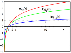
The logarithm base 10 (that is b = 10) is called the common logarithm and has many applications in science and engineering. The natural logarithm has the number e (that is b ≈ 2.718) as its base; its use is widespread in mathematics and physics, because of its simpler integral and derivative. The binary logarithm uses base 2 (that is b = 2) and is commonly used in computer science. Logarithms are examples of concave functions.[1]
Logarithms were introduced by John Napier in 1614 as a means of simplifying calculations.[2] They were rapidly adopted by navigators, scientists, engineers, surveyors and others to perform high-accuracy computations more easily. Using logarithm tables, tedious multi-digit multiplication steps can be replaced by table look-ups and simpler addition. This is possible because of the fact—important in its own right—that the logarithm of a product is the sum of the logarithms of the factors:

provided that b, x and y are all positive and b ≠ 1. The slide rule, also based on logarithms, allows quick calculations without tables, but at lower precision. The present-day notion of logarithms comes from Leonhard Euler, who connected them to the exponential function in the 18th century, and who also introduced the letter e as the base of natural logarithms.[3]
Logarithmic scales reduce wide-ranging quantities to tiny scopes. For example, the decibel (dB) is a unit used to express ratio as logarithms, mostly for signal power and amplitude (of which sound pressure is a common example). In chemistry, pH is a logarithmic measure for the acidity of an aqueous solution. Logarithms are commonplace in scientific formulae, and in measurements of the complexity of algorithms and of geometric objects called fractals. They help to describe frequency ratios of musical intervals, appear in formulas counting prime numbers or approximating factorials, inform some models in psychophysics, and can aid in forensic accounting.
In the same way as the logarithm reverses exponentiation, the complex logarithm is the inverse function of the exponential function applied to complex numbers. The modular discrete logarithm is another variant; it has uses in public-key cryptography.
Motivation and definition
Addition, multiplication, and exponentiation are three of the most fundamental arithmetic operations. Addition, the simplest of these, is undone by subtraction: when you add 5 to x to get x + 5, to reverse this operation you need to subtract 5 from x + 5. Multiplication, the next-simplest operation, is undone by division: if you multiply x by 5 to get 5x, you then must divide 5x by 5 in order to return to the original expression x. Logarithms also undo a fundamental arithmetic operation, exponentiation. Exponentiation is when you raise a number to a certain power. For example, raising 2 to the power 3 equals 8:

The general case is when you raise a number b to the power of y to get x:

The number b is referred to as the base of this expression. The base is the number that is raised to a particular power—in the above example, the base of the expression is 2. It is easy to make the base the subject of the expression: all you have to do is take the y-th root of both sides. This gives:


It is less easy to make y the subject of the expression. Logarithms allow us to do this:
- logb x

This expression means that y is equal to the power that you need to raise b to in order to get x. This operation undoes exponentiation because the logarithm of x tells you the exponent that the base has been raised to.
Exponentiation
This subsection contains a short overview of the exponentiation operation, which is fundamental to understanding logarithms. Raising b to the n-th power, where n is a natural number, is done by multiplying n factors equal to b. The n-th power of b is written bn, so that

Exponentiation may be extended to by, where b is a positive number and the exponent y is any real number.[4] For example, b−1 is the reciprocal of b, that is, 1/b. Raising b to the power 1/2 is the square root of b.
More generally, raising b to a rational power p/q, where p and q are integers, is given by

the q-th root of .

Finally, any irrational number (a real number which is not rational) y can be approximated to arbitrary precision by rational numbers. This can be used to compute the y-th power of b: for example and is increasingly well approximated by . A more detailed explanation, as well as the formula bm + n = bm · bn is contained in the article on exponentiation.


Definition
The logarithm of a positive real number x with respect to base b[nb 1] is the exponent by which b must be raised to yield x. In other words, the logarithm of x to base b is the solution y to the equation[5]

The logarithm is denoted "logb x" (pronounced as "the logarithm of x to base b" or "the base-b logarithm of x" or (most commonly) "the log, base b, of x").
In the equation y = logb x, the value y is the answer to the question "To what power must b be raised, in order to yield x?".
Examples
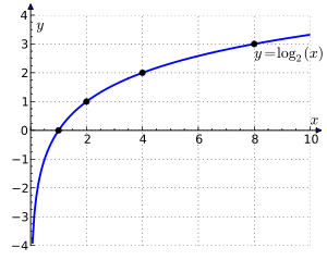
- log2 16 = 4 , since 24 = 2 ×2 × 2 × 2 = 16.
- Logarithms can also be negative: since
- log10150 is approximately 2.176, which lies between 2 and 3, just as 150 lies between 102 = 100 and 103 = 1000.
- For any base b, logb b = 1 and logb 1 = 0, since b1 = b and b0 = 1, respectively.


Logarithmic identities
Several important formulas, sometimes called logarithmic identities or logarithmic laws, relate logarithms to one another.[6]
Product, quotient, power, and root
The logarithm of a product is the sum of the logarithms of the numbers being multiplied; the logarithm of the ratio of two numbers is the difference of the logarithms. The logarithm of the p-th power of a number is p times the logarithm of the number itself; the logarithm of a p-th root is the logarithm of the number divided by p. The following table lists these identities with examples. Each of the identities can be derived after substitution of the logarithm definitions or in the left hand sides.[1]


| Formula | Example | |
|---|---|---|
| Product | ||
| Quotient | ||
| Power | ||
| Root |


Change of base
The logarithm logbx can be computed from the logarithms of x and b with respect to an arbitrary base k using the following formula:

Derivation of the conversion factor between logarithms of arbitrary base |
|---|
|
Starting from the defining identity we can apply logk to both sides of this equation, to get
Solving for yields:
showing the conversion factor from given -values to their corresponding -values to be |


Typical scientific calculators calculate the logarithms to bases 10 and e.[7] Logarithms with respect to any base b can be determined using either of these two logarithms by the previous formula:

Given a number x and its logarithm logbx to an unknown base b, the base is given by:

which can be seen from taking the defining equation to the power of

Particular bases
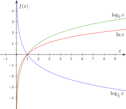
Among all choices for the base, three are particularly common. These are b = 10, b = e (the irrational mathematical constant ≈ 2.71828), and b = 2 (the binary logarithm). In mathematical analysis, the logarithm base e is widespread because of analytical properties explained below. On the other hand, base-10 logarithms are easy to use for manual calculations in the decimal number system:[8]

Thus, log10x is related to the number of decimal digits of a positive integer x: the number of digits is the smallest integer strictly bigger than log10x.[9] For example, log101430 is approximately 3.15. The next integer is 4, which is the number of digits of 1430. Both the natural logarithm and the logarithm to base two are used in information theory, corresponding to the use of nats or bits as the fundamental units of information, respectively.[10] Binary logarithms are also used in computer science, where the binary system is ubiquitous; in music theory, where a pitch ratio of two (the octave) is ubiquitous and the cent is the binary logarithm (scaled by 1200) of the ratio between two adjacent equally-tempered pitches in European classical music; and in photography to measure exposure values.[11]
The following table lists common notations for logarithms to these bases and the fields where they are used. Many disciplines write logx instead of logbx, when the intended base can be determined from the context. The notation blogx also occurs.[12] The "ISO notation" column lists designations suggested by the International Organization for Standardization (ISO 31-11).[13] Because the notation log x has been used for all three bases (or when the base is indeterminate or immaterial), the intended base must often be inferred based on context or discipline. In computer science log usually refers to log2, and in mathematics log usually refers to loge.[14][1] In other contexts log often means log10.[15]
| Base b | Name for logbx | ISO notation | Other notations | Used in |
|---|---|---|---|---|
| 2 | binary logarithm | lb x[16] | ld x, log x, lg x,[17] log2x | computer science, information theory, music theory, photography |
| e | natural logarithm | ln x[nb 2] | log x (in mathematics [1][21] and many programming languages[nb 3]) |
mathematics, physics, chemistry, statistics, economics, information theory, and engineering |
| 10 | common logarithm | lg x | log x, log10x (in engineering, biology, astronomy) |
various engineering fields (see decibel and see below), logarithm tables, handheld calculators, spectroscopy |
History
The history of logarithm in seventeenth-century Europe is the discovery of a new function that extended the realm of analysis beyond the scope of algebraic methods. The method of logarithms was publicly propounded by John Napier in 1614, in a book titled Mirifici Logarithmorum Canonis Descriptio (Description of the Wonderful Rule of Logarithms).[22][23] Prior to Napier's invention, there had been other techniques of similar scopes, such as the prosthaphaeresis or the use of tables of progressions, extensively developed by Jost Bürgi around 1600.[24][25]
The common logarithm of a number is the index of that power of ten which equals the number.[26] Speaking of a number as requiring so many figures is a rough allusion to common logarithm, and was referred to by Archimedes as the "order of a number".[27] The first real logarithms were heuristic methods to turn multiplication into addition, thus facilitating rapid computation. Some of these methods used tables derived from trigonometric identities.[28] Such methods are called prosthaphaeresis.
Invention of the function now known as natural logarithm began as an attempt to perform a quadrature of a rectangular hyperbola by Grégoire de Saint-Vincent, a Belgian Jesuit residing in Prague. Archimedes had written The Quadrature of the Parabola in the third century BC, but a quadrature for the hyperbola eluded all efforts until Saint-Vincent published his results in 1647. The relation that the logarithm provides between a geometric progression in its argument and an arithmetic progression of values, prompted A. A. de Sarasa to make the connection of Saint-Vincent's quadrature and the tradition of logarithms in prosthaphaeresis, leading to the term "hyperbolic logarithm", a synonym for natural logarithm. Soon the new function was appreciated by Christiaan Huygens, and James Gregory. The notation Log y was adopted by Leibniz in 1675,[29] and the next year he connected it to the integral

Logarithm tables, slide rules, and historical applications
By simplifying difficult calculations before calculators and computers became available, logarithms contributed to the advance of science, especially astronomy. They were critical to advances in surveying, celestial navigation, and other domains. Pierre-Simon Laplace called logarithms
- "...[a]n admirable artifice which, by reducing to a few days the labour of many months, doubles the life of the astronomer, and spares him the errors and disgust inseparable from long calculations."[30]
As the function f(x) = bx is the inverse function of logbx, it has been called the antilogarithm.[31]
Log tables
A key tool that enabled the practical use of logarithms was the table of logarithms.[32] The first such table was compiled by Henry Briggs in 1617, immediately after Napier's invention but with the innovation of using 10 as the base. Briggs' first table contained the common logarithms of all integers in the range 1–1000, with a precision of 14 digits. Subsequently, tables with increasing scope were written. These tables listed the values of log10x for any number x in a certain range, at a certain precision. Base-10 logarithms were universally used for computation, hence the name common logarithm, since numbers that differ by factors of 10 have logarithms that differ by integers. The common logarithm of x can be separated into an integer part and a fractional part, known as the characteristic and mantissa. Tables of logarithms need only include the mantissa, as the characteristic can be easily determined by counting digits from the decimal point.[33] The characteristic of 10 · x is one plus the characteristic of x, and their mantissas are the same. Thus using a three-digit log table, the logarithm of 3542 is approximated by

Greater accuracy can be obtained by interpolation:

The value of 10x can be determined by reverse look up in the same table, since the logarithm is a monotonic function.
Computations
The product and quotient of two positive numbers c and d were routinely calculated as the sum and difference of their logarithms. The product cd or quotient c/d came from looking up the antilogarithm of the sum or difference, via the same table:

and

For manual calculations that demand any appreciable precision, performing the lookups of the two logarithms, calculating their sum or difference, and looking up the antilogarithm is much faster than performing the multiplication by earlier methods such as prosthaphaeresis, which relies on trigonometric identities.
Calculations of powers and roots are reduced to multiplications or divisions and look-ups by

and

Trigonometric calculations were facilitated by tables that contained the common logarithms of trigonometric functions.
Slide rules
Another critical application was the slide rule, a pair of logarithmically divided scales used for calculation. The non-sliding logarithmic scale, Gunter's rule, was invented shortly after Napier's invention. William Oughtred enhanced it to create the slide rule—a pair of logarithmic scales movable with respect to each other. Numbers are placed on sliding scales at distances proportional to the differences between their logarithms. Sliding the upper scale appropriately amounts to mechanically adding logarithms, as illustrated here:
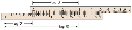
For example, adding the distance from 1 to 2 on the lower scale to the distance from 1 to 3 on the upper scale yields a product of 6, which is read off at the lower part. The slide rule was an essential calculating tool for engineers and scientists until the 1970s, because it allows, at the expense of precision, much faster computation than techniques based on tables.[34]
Analytic properties
A deeper study of logarithms requires the concept of a function. A function is a rule that, given one number, produces another number.[35] An example is the function producing the x-th power of b from any real number x, where the base b is a fixed number. This function is written:

Logarithmic function
To justify the definition of logarithms, it is necessary to show that the equation

has a solution x and that this solution is unique, provided that y is positive and that b is positive and unequal to 1. A proof of that fact requires the intermediate value theorem from elementary calculus.[36] This theorem states that a continuous function that produces two values m and n also produces any value that lies between m and n. A function is continuous if it does not "jump", that is, if its graph can be drawn without lifting the pen.
This property can be shown to hold for the function f(x) = bx. Because f takes arbitrarily large and arbitrarily small positive values, any number y > 0 lies between f(x0) and f(x1) for suitable x0 and x1. Hence, the intermediate value theorem ensures that the equation f(x) = y has a solution. Moreover, there is only one solution to this equation, because the function f is strictly increasing (for b > 1), or strictly decreasing (for 0 < b < 1).[37]
The unique solution x is the logarithm of y to base b, logby. The function that assigns to y its logarithm is called logarithm function or logarithmic function (or just logarithm).
The function logbx is essentially characterized by the product formula

More precisely, the logarithm to any base b > 1 is the only increasing function f from the positive reals to the reals satisfying f(b) = 1 and [38]

Inverse function

The formula for the logarithm of a power says in particular that for any number x,

In prose, taking the x-th power of b and then the base-b logarithm gives back x. Conversely, given a positive number y, the formula

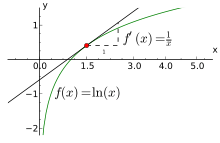
says that first taking the logarithm and then exponentiating gives back y. Thus, the two possible ways of combining (or composing) logarithms and exponentiation give back the original number. Therefore, the logarithm to base b is the inverse function of f(x) = bx.[39]
Inverse functions are closely related to the original functions. Their graphs correspond to each other upon exchanging the x- and the y-coordinates (or upon reflection at the diagonal line x = y), as shown at the right: a point (t, u = bt) on the graph of f yields a point (u, t = logbu) on the graph of the logarithm and vice versa. As a consequence, logb(x) diverges to infinity (gets bigger than any given number) if x grows to infinity, provided that b is greater than one. In that case, logb(x) is an increasing function. For b < 1, logb(x) tends to minus infinity instead. When x approaches zero, logbx goes to minus infinity for b > 1 (plus infinity for b < 1, respectively).
Derivative and antiderivative
Analytic properties of functions pass to their inverses.[36] Thus, as f(x) = bx is a continuous and differentiable function, so is logby. Roughly, a continuous function is differentiable if its graph has no sharp "corners". Moreover, as the derivative of f(x) evaluates to ln(b)bx by the properties of the exponential function, the chain rule implies that the derivative of logbx is given by[37][40]

That is, the slope of the tangent touching the graph of the base-b logarithm at the point (x, logb(x)) equals 1/(x ln(b)).
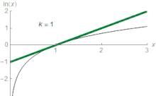
The derivative of ln x is 1/x; this implies that ln x is the unique antiderivative of 1/x that has the value 0 for x =1. It is this very simple formula that motivated to qualify as "natural" the natural logarithm; this is also one of the main reasons of the importance of the constant e.
The derivative with a generalised functional argument f(x) is

The quotient at the right hand side is called the logarithmic derivative of f. Computing f'(x) by means of the derivative of ln(f(x)) is known as logarithmic differentiation.[41] The antiderivative of the natural logarithm ln(x) is:[42]

Related formulas, such as antiderivatives of logarithms to other bases can be derived from this equation using the change of bases.[43]
Integral representation of the natural logarithm
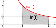
The natural logarithm of t equals the integral of 1/x dx from 1 to t:

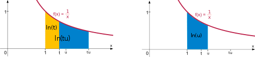
In other words, ln(t) equals the area between the x axis and the graph of the function 1/x, ranging from x = 1 to x = t (figure at the right). This is a consequence of the fundamental theorem of calculus and the fact that the derivative of ln(x) is 1/x. The right hand side of this equation can serve as a definition of the natural logarithm. Product and power logarithm formulas can be derived from this definition.[44] For example, the product formula ln(tu) = ln(t) + ln(u) is deduced as:

The equality (1) splits the integral into two parts, while the equality (2) is a change of variable (w = x/t). In the illustration below, the splitting corresponds to dividing the area into the yellow and blue parts. Rescaling the left hand blue area vertically by the factor t and shrinking it by the same factor horizontally does not change its size. Moving it appropriately, the area fits the graph of the function f(x) = 1/x again. Therefore, the left hand blue area, which is the integral of f(x) from t to tu is the same as the integral from 1 to u. This justifies the equality (2) with a more geometric proof.
The power formula ln(tr) = r ln(t) may be derived in a similar way:

The second equality uses a change of variables (integration by substitution), w = x1/r.
The sum over the reciprocals of natural numbers,

is called the harmonic series. It is closely tied to the natural logarithm: as n tends to infinity, the difference,

converges (i.e., gets arbitrarily close) to a number known as the Euler–Mascheroni constant γ = 0.5772.... This relation aids in analyzing the performance of algorithms such as quicksort.[45]
There are also some other integral representations of the logarithm that are useful in some situations:


The first identity can be verified by showing that it has the same value at x = 1, and the same derivative. The second identity can be proven by writing

and then inserting the Laplace transform of cos(xt) (and cos(t)).
Transcendence of the logarithm
Real numbers that are not algebraic are called transcendental;[46] for example, π and e are such numbers, but is not. Almost all real numbers are transcendental. The logarithm is an example of a transcendental function. The Gelfond–Schneider theorem asserts that logarithms usually take transcendental, i.e., "difficult" values.[47]

Calculation
Logarithms are easy to compute in some cases, such as log10(1000) = 3. In general, logarithms can be calculated using power series or the arithmetic–geometric mean, or be retrieved from a precalculated logarithm table that provides a fixed precision.[48][49] Newton's method, an iterative method to solve equations approximately, can also be used to calculate the logarithm, because its inverse function, the exponential function, can be computed efficiently.[50] Using look-up tables, CORDIC-like methods can be used to compute logarithms if the only available operations are addition and bit shifts.[51][52] Moreover, the binary logarithm algorithm calculates lb(x) recursively based on repeated squarings of x, taking advantage of the relation

Power series
- Taylor series
For any real number z that satisfies 0 < z < 2, the following formula holds:[nb 4][53]

This is a shorthand for saying that ln(z) can be approximated to a more and more accurate value by the following expressions:

For example, with z = 1.5 the third approximation yields 0.4167, which is about 0.011 greater than ln(1.5) = 0.405465. This series approximates ln(z) with arbitrary precision, provided the number of summands is large enough. In elementary calculus, ln(z) is therefore the limit of this series. It is the Taylor series of the natural logarithm at z = 1. The Taylor series of ln(z) provides a particularly useful approximation to ln(1+z) when z is small, |z| < 1, since then

For example, with z = 0.1 the first-order approximation gives ln(1.1) ≈ 0.1, which is less than 5% off the correct value 0.0953.
- More efficient series
Another series is based on the area hyperbolic tangent function:

for any real number z > 0.[nb 5][53] Using sigma notation, this is also written as

This series can be derived from the above Taylor series. It converges more quickly than the Taylor series, especially if z is close to 1. For example, for z = 1.5, the first three terms of the second series approximate ln(1.5) with an error of about 3×10⁻⁶. The quick convergence for z close to 1 can be taken advantage of in the following way: given a low-accuracy approximation y ≈ ln(z) and putting

the logarithm of z is:

The better the initial approximation y is, the closer A is to 1, so its logarithm can be calculated efficiently. A can be calculated using the exponential series, which converges quickly provided y is not too large. Calculating the logarithm of larger z can be reduced to smaller values of z by writing z = a · 10b, so that ln(z) = ln(a) + b · ln(10).
A closely related method can be used to compute the logarithm of integers. Putting in the above series, it follows that:


If the logarithm of a large integer n is known, then this series yields a fast converging series for log(n+1), with a rate of convergence of .

Arithmetic–geometric mean approximation
The arithmetic–geometric mean yields high precision approximations of the natural logarithm. Sasaki and Kanada showed in 1982 that it was particularly fast for precisions between 400 and 1000 decimal places, while Taylor series methods were typically faster when less precision was needed. In their work ln(x) is approximated to a precision of 2−p (or p precise bits) by the following formula (due to Carl Friedrich Gauss):[54][55]

Here M(x,y) denotes the arithmetic–geometric mean of x and y. It is obtained by repeatedly calculating the average (arithmetic mean) and (geometric mean) of x and y then let those two numbers become the next x and y. The two numbers quickly converge to a common limit which is the value of M(x,y). m is chosen such that


to ensure the required precision. A larger m makes the M(x,y) calculation take more steps (the initial x and y are farther apart so it takes more steps to converge) but gives more precision. The constants pi and ln(2) can be calculated with quickly converging series.
Feynman's algorithm
While at Los Alamos National Laboratory working on the Manhattan Project, Richard Feynman developed a bit-processing algorithm that is similar to long division and was later used in the Connection Machine. The algorithm uses the fact that every real number is representable as a product of distinct factors of the form . The algorithm sequentially builds that product : if , then it changes to . It then increase by one regardless. The algorithm stops when is large enough to give the desired accuracy. Because is the sum of the terms of the form corresponding to those for which the factor was included in the product , may be computed by simple addition, using a table of for all . Any base may be used for the logarithm table.[56]


Applications
Logarithms have many applications inside and outside mathematics. Some of these occurrences are related to the notion of scale invariance. For example, each chamber of the shell of a nautilus is an approximate copy of the next one, scaled by a constant factor. This gives rise to a logarithmic spiral.[57] Benford's law on the distribution of leading digits can also be explained by scale invariance.[58] Logarithms are also linked to self-similarity. For example, logarithms appear in the analysis of algorithms that solve a problem by dividing it into two similar smaller problems and patching their solutions.[59] The dimensions of self-similar geometric shapes, that is, shapes whose parts resemble the overall picture are also based on logarithms. Logarithmic scales are useful for quantifying the relative change of a value as opposed to its absolute difference. Moreover, because the logarithmic function log(x) grows very slowly for large x, logarithmic scales are used to compress large-scale scientific data. Logarithms also occur in numerous scientific formulas, such as the Tsiolkovsky rocket equation, the Fenske equation, or the Nernst equation.
Logarithmic scale
Scientific quantities are often expressed as logarithms of other quantities, using a logarithmic scale. For example, the decibel is a unit of measurement associated with logarithmic-scale quantities. It is based on the common logarithm of ratios—10 times the common logarithm of a power ratio or 20 times the common logarithm of a voltage ratio. It is used to quantify the loss of voltage levels in transmitting electrical signals,[60] to describe power levels of sounds in acoustics,[61] and the absorbance of light in the fields of spectrometry and optics. The signal-to-noise ratio describing the amount of unwanted noise in relation to a (meaningful) signal is also measured in decibels.[62] In a similar vein, the peak signal-to-noise ratio is commonly used to assess the quality of sound and image compression methods using the logarithm.[63]
The strength of an earthquake is measured by taking the common logarithm of the energy emitted at the quake. This is used in the moment magnitude scale or the Richter magnitude scale. For example, a 5.0 earthquake releases 32 times (101.5) and a 6.0 releases 1000 times (103) the energy of a 4.0.[64] Another logarithmic scale is apparent magnitude. It measures the brightness of stars logarithmically.[65] Yet another example is pH in chemistry; pH is the negative of the common logarithm of the activity of hydronium ions (the form hydrogen ions H+
take in water).[66] The activity of hydronium ions in neutral water is 10−7 mol·L−1, hence a pH of 7. Vinegar typically has a pH of about 3. The difference of 4 corresponds to a ratio of 104 of the activity, that is, vinegar's hydronium ion activity is about 10−3 mol·L−1.
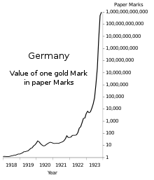
Semilog (log-linear) graphs use the logarithmic scale concept for visualization: one axis, typically the vertical one, is scaled logarithmically. For example, the chart at the right compresses the steep increase from 1 million to 1 trillion to the same space (on the vertical axis) as the increase from 1 to 1 million. In such graphs, exponential functions of the form f(x) = a · bx appear as straight lines with slope equal to the logarithm of b. Log-log graphs scale both axes logarithmically, which causes functions of the form f(x) = a · xk to be depicted as straight lines with slope equal to the exponent k. This is applied in visualizing and analyzing power laws.[67]
Psychology
Logarithms occur in several laws describing human perception:[68][69] Hick's law proposes a logarithmic relation between the time individuals take to choose an alternative and the number of choices they have.[70] Fitts's law predicts that the time required to rapidly move to a target area is a logarithmic function of the distance to and the size of the target.[71] In psychophysics, the Weber–Fechner law proposes a logarithmic relationship between stimulus and sensation such as the actual vs. the perceived weight of an item a person is carrying.[72] (This "law", however, is less realistic than more recent models, such as Stevens's power law.[73])
Psychological studies found that individuals with little mathematics education tend to estimate quantities logarithmically, that is, they position a number on an unmarked line according to its logarithm, so that 10 is positioned as close to 100 as 100 is to 1000. Increasing education shifts this to a linear estimate (positioning 1000 10x as far away) in some circumstances, while logarithms are used when the numbers to be plotted are difficult to plot linearly.[74][75]
Probability theory and statistics
Logarithms arise in probability theory: the law of large numbers dictates that, for a fair coin, as the number of coin-tosses increases to infinity, the observed proportion of heads approaches one-half. The fluctuations of this proportion about one-half are described by the law of the iterated logarithm.[76]
Logarithms also occur in log-normal distributions. When the logarithm of a random variable has a normal distribution, the variable is said to have a log-normal distribution.[77] Log-normal distributions are encountered in many fields, wherever a variable is formed as the product of many independent positive random variables, for example in the study of turbulence.[78]
Logarithms are used for maximum-likelihood estimation of parametric statistical models. For such a model, the likelihood function depends on at least one parameter that must be estimated. A maximum of the likelihood function occurs at the same parameter-value as a maximum of the logarithm of the likelihood (the "log likelihood"), because the logarithm is an increasing function. The log-likelihood is easier to maximize, especially for the multiplied likelihoods for independent random variables.[79]
Benford's law describes the occurrence of digits in many data sets, such as heights of buildings. According to Benford's law, the probability that the first decimal-digit of an item in the data sample is d (from 1 to 9) equals log10(d + 1) − log10(d), regardless of the unit of measurement.[80] Thus, about 30% of the data can be expected to have 1 as first digit, 18% start with 2, etc. Auditors examine deviations from Benford's law to detect fraudulent accounting.[81]
Computational complexity
Analysis of algorithms is a branch of computer science that studies the performance of algorithms (computer programs solving a certain problem).[82] Logarithms are valuable for describing algorithms that divide a problem into smaller ones, and join the solutions of the subproblems.[83]
For example, to find a number in a sorted list, the binary search algorithm checks the middle entry and proceeds with the half before or after the middle entry if the number is still not found. This algorithm requires, on average, log2(N) comparisons, where N is the list's length.[84] Similarly, the merge sort algorithm sorts an unsorted list by dividing the list into halves and sorting these first before merging the results. Merge sort algorithms typically require a time approximately proportional to N · log(N).[85] The base of the logarithm is not specified here, because the result only changes by a constant factor when another base is used. A constant factor is usually disregarded in the analysis of algorithms under the standard uniform cost model.[86]
A function f(x) is said to grow logarithmically if f(x) is (exactly or approximately) proportional to the logarithm of x. (Biological descriptions of organism growth, however, use this term for an exponential function.[87]) For example, any natural number N can be represented in binary form in no more than log2(N) + 1 bits. In other words, the amount of memory needed to store N grows logarithmically with N.
Entropy and chaos

Entropy is broadly a measure of the disorder of some system. In statistical thermodynamics, the entropy S of some physical system is defined as

The sum is over all possible states i of the system in question, such as the positions of gas particles in a container. Moreover, pi is the probability that the state i is attained and k is the Boltzmann constant. Similarly, entropy in information theory measures the quantity of information. If a message recipient may expect any one of N possible messages with equal likelihood, then the amount of information conveyed by any one such message is quantified as log2(N) bits.[88]
Lyapunov exponents use logarithms to gauge the degree of chaoticity of a dynamical system. For example, for a particle moving on an oval billiard table, even small changes of the initial conditions result in very different paths of the particle. Such systems are chaotic in a deterministic way, because small measurement errors of the initial state predictably lead to largely different final states.[89] At least one Lyapunov exponent of a deterministically chaotic system is positive.
Fractals

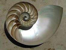
Logarithms occur in definitions of the dimension of fractals.[90] Fractals are geometric objects that are self-similar: small parts reproduce, at least roughly, the entire global structure. The Sierpinski triangle (pictured) can be covered by three copies of itself, each having sides half the original length. This makes the Hausdorff dimension of this structure ln(3)/ln(2) ≈ 1.58. Another logarithm-based notion of dimension is obtained by counting the number of boxes needed to cover the fractal in question.
Music
Logarithms are related to musical tones and intervals. In equal temperament, the frequency ratio depends only on the interval between two tones, not on the specific frequency, or pitch, of the individual tones. For example, the note A has a frequency of 440 Hz and B-flat has a frequency of 466 Hz. The interval between A and B-flat is a semitone, as is the one between B-flat and B (frequency 493 Hz). Accordingly, the frequency ratios agree:

Therefore, logarithms can be used to describe the intervals: an interval is measured in semitones by taking the base-21/12 logarithm of the frequency ratio, while the base-21/1200 logarithm of the frequency ratio expresses the interval in cents, hundredths of a semitone. The latter is used for finer encoding, as it is needed for non-equal temperaments.[91]
| Interval (the two tones are played at the same time) |
1/12 tone |
Semitone |
Just major third |
Major third |
Tritone |
Octave |
| Frequency ratio r | ||||||
| Corresponding number of semitones |
||||||
| Corresponding number of cents |


Number theory
Natural logarithms are closely linked to counting prime numbers (2, 3, 5, 7, 11, ...), an important topic in number theory. For any integer x, the quantity of prime numbers less than or equal to x is denoted π(x). The prime number theorem asserts that π(x) is approximately given by

in the sense that the ratio of π(x) and that fraction approaches 1 when x tends to infinity.[92] As a consequence, the probability that a randomly chosen number between 1 and x is prime is inversely proportional to the number of decimal digits of x. A far better estimate of π(x) is given by the offset logarithmic integral function Li(x), defined by

The Riemann hypothesis, one of the oldest open mathematical conjectures, can be stated in terms of comparing π(x) and Li(x).[93] The Erdős–Kac theorem describing the number of distinct prime factors also involves the natural logarithm.
The logarithm of n factorial, n! = 1 · 2 · ... · n, is given by

This can be used to obtain Stirling's formula, an approximation of n! for large n.[94]
Generalizations
Complex logarithm

All the complex numbers a that solve the equation

are called complex logarithms of z, when z is (considered as) a complex number. A complex number is commonly represented as z = x + iy, where x and y are real numbers and i is an imaginary unit, the square of which is −1. Such a number can be visualized by a point in the complex plane, as shown at the right. The polar form encodes a non-zero complex number z by its absolute value, that is, the (positive, real) distance r to the origin, and an angle between the real (x) axis Re and the line passing through both the origin and z. This angle is called the argument of z.
The absolute value r of z is given by

Using the geometrical interpretation of and and their periodicity in any complex number z may be denoted as


for any integer number k. Evidently the argument of z is not uniquely specified: both φ and φ' = φ + 2kπ are valid arguments of z for all integers k, because adding 2kπ radian or k⋅360°[nb 6] to φ corresponds to "winding" around the origin counter-clock-wise by k turns. The resulting complex number is always z, as illustrated at the right for k = 1. One may select exactly one of the possible arguments of z as the so-called principal argument, denoted Arg(z), with a capital A, by requiring φ to belong to one, conveniently selected turn, e.g., [95] or [96] These regions, where the argument of z is uniquely determined are called branches of the argument function.


Euler's formula connects the trigonometric functions sine and cosine to the complex exponential:

Using this formula, and again the periodicity, the following identities hold:[97]

where ln(r) is the unique real natural logarithm, ak denote the complex logarithms of z, and k is an arbitrary integer. Therefore, the complex logarithms of z, which are all those complex values ak for which the ak-th power of e equals z, are the infinitely many values
- for arbitrary integers k.

Taking k such that is within the defined interval for the principal arguments, then ak is called the principal value of the logarithm, denoted Log(z), again with a capital L. The principal argument of any positive real number x is 0; hence Log(x) is a real number and equals the real (natural) logarithm. However, the above formulas for logarithms of products and powers do not generalize to the principal value of the complex logarithm.[98]

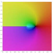
The illustration at the right depicts Log(z), confining the arguments of z to the interval (-π, π]. This way the corresponding branch of the complex logarithm has discontinuities all along the negative real x axis, which can be seen in the jump in the hue there. This discontinuity arises from jumping to the other boundary in the same branch, when crossing a boundary, i.e., not changing to the corresponding k-value of the continuously neighboring branch. Such a locus is called a branch cut. Dropping the range restrictions on the argument makes the relations "argument of z", and consequently the "logarithm of z", multi-valued functions.
Inverses of other exponential functions
Exponentiation occurs in many areas of mathematics and its inverse function is often referred to as the logarithm. For example, the logarithm of a matrix is the (multi-valued) inverse function of the matrix exponential.[99] Another example is the p-adic logarithm, the inverse function of the p-adic exponential. Both are defined via Taylor series analogous to the real case.[100] In the context of differential geometry, the exponential map maps the tangent space at a point of a manifold to a neighborhood of that point. Its inverse is also called the logarithmic (or log) map.[101]
In the context of finite groups exponentiation is given by repeatedly multiplying one group element b with itself. The discrete logarithm is the integer n solving the equation

where x is an element of the group. Carrying out the exponentiation can be done efficiently, but the discrete logarithm is believed to be very hard to calculate in some groups. This asymmetry has important applications in public key cryptography, such as for example in the Diffie–Hellman key exchange, a routine that allows secure exchanges of cryptographic keys over unsecured information channels.[102] Zech's logarithm is related to the discrete logarithm in the multiplicative group of non-zero elements of a finite field.[103]
Further logarithm-like inverse functions include the double logarithm ln(ln(x)), the super- or hyper-4-logarithm (a slight variation of which is called iterated logarithm in computer science), the Lambert W function, and the logit. They are the inverse functions of the double exponential function, tetration, of f(w) = wew,[104] and of the logistic function, respectively.[105]
Related concepts
From the perspective of group theory, the identity log(cd) = log(c) + log(d) expresses a group isomorphism between positive reals under multiplication and reals under addition. Logarithmic functions are the only continuous isomorphisms between these groups.[106] By means of that isomorphism, the Haar measure (Lebesgue measure) dx on the reals corresponds to the Haar measure dx/x on the positive reals.[107] The non-negative reals not only have a multiplication, but also have addition, and form a semiring, called the probability semiring; this is in fact a semifield. The logarithm then takes multiplication to addition (log multiplication), and takes addition to log addition (LogSumExp), giving an isomorphism of semirings between the probability semiring and the log semiring.
Logarithmic one-forms df/f appear in complex analysis and algebraic geometry as differential forms with logarithmic poles.[108]
The polylogarithm is the function defined by

It is related to the natural logarithm by Li1(z) = −ln(1 − z). Moreover, Lis(1) equals the Riemann zeta function ζ(s).[109]
See also
- Cologarithm
- Decimal exponent (dex)
- Exponential function
- Index of logarithm articles
- Logarithmic notation
Notes
- The restrictions on x and b are explained in the section "Analytic properties".
- Some mathematicians disapprove of this notation. In his 1985 autobiography, Paul Halmos criticized what he considered the "childish ln notation," which he said no mathematician had ever used.[18] The notation was invented by Irving Stringham, a mathematician.[19][20]
- For example C, Java, Haskell, and BASIC.
- The same series holds for the principal value of the complex logarithm for complex numbers z satisfying |z − 1| < 1.
- The same series holds for the principal value of the complex logarithm for complex numbers z with positive real part.
- See radian for the conversion between 2π and 360 degree.
References
- "The Ultimate Guide to Logarithm — Theory & Applications". Math Vault. 8 May 2016. Retrieved 24 July 2019.
- Hobson, Ernest William (1914). John Napier and the invention of logarithms, 1614; a lecture. University of California Libraries. Cambridge : University Press.
- Remmert, Reinhold. (1991). Theory of complex functions. New York: Springer-Verlag. ISBN 0387971955. OCLC 21118309.
- Shirali, Shailesh (2002), A Primer on Logarithms, Hyderabad: Universities Press, ISBN 978-81-7371-414-6, esp. section 2
- Kate, S.K.; Bhapkar, H.R. (2009), Basics Of Mathematics, Pune: Technical Publications, ISBN 978-81-8431-755-8, chapter 1
- All statements in this section can be found in Shailesh Shirali 2002, section 4, (Douglas Downing 2003, p. 275), or Kate & Bhapkar 2009, p. 1-1, for example.
- Bernstein, Stephen; Bernstein, Ruth (1999), Schaum's outline of theory and problems of elements of statistics. I, Descriptive statistics and probability, Schaum's outline series, New York: McGraw-Hill, ISBN 978-0-07-005023-5, p. 21
- Downing, Douglas (2003), Algebra the Easy Way, Barron's Educational Series, Hauppauge, NY: Barron's, ISBN 978-0-7641-1972-9, chapter 17, p. 275
- Wegener, Ingo (2005), Complexity theory: exploring the limits of efficient algorithms, Berlin, New York: Springer-Verlag, ISBN 978-3-540-21045-0, p. 20
- Van der Lubbe, Jan C. A. (1997), Information Theory, Cambridge University Press, p. 3, ISBN 978-0-521-46760-5
- Allen, Elizabeth; Triantaphillidou, Sophie (2011), The Manual of Photography, Taylor & Francis, p. 228, ISBN 978-0-240-52037-7
- Franz Embacher; Petra Oberhuemer, Mathematisches Lexikon (in German), mathe online: für Schule, Fachhochschule, Universität unde Selbststudium, retrieved 22 March 2011
- Taylor, B.N. (1995), Guide for the Use of the International System of Units (SI), US Department of Commerce, archived from the original on 29 June 2007, retrieved 25 May 2007
- Goodrich, Michael T.; Tamassia, Roberto (2002), Algorithm Design: Foundations, Analysis, and Internet Examples, John Wiley & Sons, p. 23,
One of the interesting and sometimes even surprising aspects of the analysis of data structures and algorithms is the ubiquitous presence of logarithms ... As is the custom in the computing literature, we omit writing the base b of the logarithm when b = 2.
- Parkhurst, David F. (2007). Introduction to Applied Mathematics for Environmental Science (illustrated ed.). Springer Science & Business Media. p. 288. ISBN 978-0-387-34228-3.
- Gullberg, Jan (1997), Mathematics: from the birth of numbers., New York: W. W. Norton & Co, ISBN 978-0-393-04002-9
- See footnote 1 in Perl, Yehoshua; Reingold, Edward M. (December 1977). "Understanding the complexity of interpolation search". Information Processing Letters. 6 (6): 219–22. doi:10.1016/0020-0190(77)90072-2.
- Paul Halmos (1985), I Want to Be a Mathematician: An Automathography, Berlin, New York: Springer-Verlag, ISBN 978-0-387-96078-4
- Irving Stringham (1893), Uniplanar algebra: being part I of a propædeutic to the higher mathematical analysis, The Berkeley Press, p. xiii
- Roy S. Freedman (2006), Introduction to Financial Technology, Amsterdam: Academic Press, p. 59, ISBN 978-0-12-370478-8
- See Theorem 3.29 in Rudin, Walter (1984). Principles of mathematical analysis (3rd ed., International student ed.). Auckland: McGraw-Hill International. ISBN 978-0-07-085613-4.
- Napier, John (1614), Mirifici Logarithmorum Canonis Descriptio [The Description of the Wonderful Rule of Logarithms] (in Latin), Edinburgh, Scotland: Andrew Hart
- Hobson, Ernest William (1914), John Napier and the invention of logarithms, 1614, Cambridge: The University Press
- Folkerts, Menso; Launert, Dieter; Thom, Andreas (October 2015), Jost Bürgi's Method for Calculating Sines, arXiv:1510.03180, Bibcode:2015arXiv151003180F
- "Burgi biography". www-history.mcs.st-and.ac.uk. Retrieved 14 February 2018.
- William Gardner (1742) Tables of Logarithms
- R.C. Pierce (1977) "A brief history of logarithm", Two-Year College Mathematics Journal 8(1):22–26.
- Enrique Gonzales-Velasco (2011) Journey through Mathematics – Creative Episodes in its History, §2.4 Hyperbolic logarithms, p. 117, Springer ISBN 978-0-387-92153-2
- Florian Cajori (1913) "History of the exponential and logarithm concepts", American Mathematical Monthly 20: 5, 35, 75, 107, 148, 173, 205.
- Bryant, Walter W. (1907), A History of Astronomy, London: Methuen & Co, p. 44
- Abramowitz, Milton; Stegun, Irene A., eds. (1972), Handbook of Mathematical Functions with Formulas, Graphs, and Mathematical Tables (10th ed.), New York: Dover Publications, ISBN 978-0-486-61272-0, section 4.7., p. 89
- Campbell-Kelly, Martin (2003), The history of mathematical tables: from Sumer to spreadsheets, Oxford scholarship online, Oxford University Press, ISBN 978-0-19-850841-0, section 2
- Spiegel, Murray R.; Moyer, R.E. (2006), Schaum's outline of college algebra, Schaum's outline series, New York: McGraw-Hill, ISBN 978-0-07-145227-4, p. 264
- Maor 2009, sections 1, 13
- Devlin, Keith (2004). Sets, functions, and logic: an introduction to abstract mathematics. Chapman & Hall/CRC mathematics (3rd ed.). Boca Raton, Fla: Chapman & Hall/CRC. ISBN 978-1-58488-449-1., or see the references in function
- Lang, Serge (1997), Undergraduate analysis, Undergraduate Texts in Mathematics (2nd ed.), Berlin, New York: Springer-Verlag, doi:10.1007/978-1-4757-2698-5, ISBN 978-0-387-94841-6, MR 1476913, section III.3
- Lang 1997, section IV.2
- Dieudonné, Jean (1969). Foundations of Modern Analysis. 1. Academic Press. p. 84. item (4.3.1)
- Stewart, James (2007), Single Variable Calculus: Early Transcendentals, Belmont: Thomson Brooks/Cole, ISBN 978-0-495-01169-9, section 1.6
- "Calculation of d/dx(Log(b,x))". Wolfram Alpha. Wolfram Research. Retrieved 15 March 2011.
- Kline, Morris (1998), Calculus: an intuitive and physical approach, Dover books on mathematics, New York: Dover Publications, ISBN 978-0-486-40453-0, p. 386
- "Calculation of Integrate(ln(x))". Wolfram Alpha. Wolfram Research. Retrieved 15 March 2011.
- Abramowitz & Stegun, eds. 1972, p. 69
- Courant, Richard (1988), Differential and integral calculus. Vol. I, Wiley Classics Library, New York: John Wiley & Sons, ISBN 978-0-471-60842-4, MR 1009558, section III.6
- Havil, Julian (2003), Gamma: Exploring Euler's Constant, Princeton University Press, ISBN 978-0-691-09983-5, sections 11.5 and 13.8
- Nomizu, Katsumi (1996), Selected papers on number theory and algebraic geometry, 172, Providence, RI: AMS Bookstore, p. 21, ISBN 978-0-8218-0445-2
- Baker, Alan (1975), Transcendental number theory, Cambridge University Press, ISBN 978-0-521-20461-3, p. 10
- Muller, Jean-Michel (2006), Elementary functions (2nd ed.), Boston, MA: Birkhäuser Boston, ISBN 978-0-8176-4372-0, sections 4.2.2 (p. 72) and 5.5.2 (p. 95)
- Hart; Cheney; Lawson; et al. (1968), Computer Approximations, SIAM Series in Applied Mathematics, New York: John Wiley, section 6.3, pp. 105–11
- Zhang, M.; Delgado-Frias, J.G.; Vassiliadis, S. (1994), "Table driven Newton scheme for high precision logarithm generation", IEE Proceedings - Computers and Digital Techniques, 141 (5): 281–92, doi:10.1049/ip-cdt:19941268, ISSN 1350-2387, section 1 for an overview
- Meggitt, J.E. (April 1962), "Pseudo Division and Pseudo Multiplication Processes", IBM Journal of Research and Development, 6 (2): 210–26, doi:10.1147/rd.62.0210
- Kahan, W. (20 May 2001), Pseudo-Division Algorithms for Floating-Point Logarithms and Exponentials
- Abramowitz & Stegun, eds. 1972, p. 68
- Sasaki, T.; Kanada, Y. (1982), "Practically fast multiple-precision evaluation of log(x)", Journal of Information Processing, 5 (4): 247–50, retrieved 30 March 2011
- Ahrendt, Timm (1999), "Fast Computations of the Exponential Function", Stacs 99, Lecture notes in computer science, 1564, Berlin, New York: Springer, pp. 302–12, doi:10.1007/3-540-49116-3_28, ISBN 978-3-540-65691-3
- Hillis, Danny (15 January 1989). "Richard Feynman and The Connection Machine". Physics Today. 42 (2): 78. Bibcode:1989PhT....42b..78H. doi:10.1063/1.881196.
- Maor 2009, p. 135
- Frey, Bruce (2006), Statistics hacks, Hacks Series, Sebastopol, CA: O'Reilly, ISBN 978-0-596-10164-0, chapter 6, section 64
- Ricciardi, Luigi M. (1990), Lectures in applied mathematics and informatics, Manchester: Manchester University Press, ISBN 978-0-7190-2671-3, p. 21, section 1.3.2
- Bakshi, U.A. (2009), Telecommunication Engineering, Pune: Technical Publications, ISBN 978-81-8431-725-1, section 5.2
- Maling, George C. (2007), "Noise", in Rossing, Thomas D. (ed.), Springer handbook of acoustics, Berlin, New York: Springer-Verlag, ISBN 978-0-387-30446-5, section 23.0.2
- Tashev, Ivan Jelev (2009), Sound Capture and Processing: Practical Approaches, New York: John Wiley & Sons, p. 98, ISBN 978-0-470-31983-3
- Chui, C.K. (1997), Wavelets: a mathematical tool for signal processing, SIAM monographs on mathematical modeling and computation, Philadelphia: Society for Industrial and Applied Mathematics, ISBN 978-0-89871-384-8
- Crauder, Bruce; Evans, Benny; Noell, Alan (2008), Functions and Change: A Modeling Approach to College Algebra (4th ed.), Boston: Cengage Learning, ISBN 978-0-547-15669-9, section 4.4.
- Bradt, Hale (2004), Astronomy methods: a physical approach to astronomical observations, Cambridge Planetary Science, Cambridge University Press, ISBN 978-0-521-53551-9, section 8.3, p. 231
- IUPAC (1997), A. D. McNaught, A. Wilkinson (ed.), Compendium of Chemical Terminology ("Gold Book") (2nd ed.), Oxford: Blackwell Scientific Publications, doi:10.1351/goldbook, ISBN 978-0-9678550-9-7
- Bird, J.O. (2001), Newnes engineering mathematics pocket book (3rd ed.), Oxford: Newnes, ISBN 978-0-7506-4992-6, section 34
- Goldstein, E. Bruce (2009), Encyclopedia of Perception, Encyclopedia of Perception, Thousand Oaks, CA: Sage, ISBN 978-1-4129-4081-8, pp. 355–56
- Matthews, Gerald (2000), Human performance: cognition, stress, and individual differences, Human Performance: Cognition, Stress, and Individual Differences, Hove: Psychology Press, ISBN 978-0-415-04406-6, p. 48
- Welford, A.T. (1968), Fundamentals of skill, London: Methuen, ISBN 978-0-416-03000-6, OCLC 219156, p. 61
- Paul M. Fitts (June 1954), "The information capacity of the human motor system in controlling the amplitude of movement", Journal of Experimental Psychology, 47 (6): 381–91, doi:10.1037/h0055392, PMID 13174710, reprinted in Paul M. Fitts (1992), "The information capacity of the human motor system in controlling the amplitude of movement" (PDF), Journal of Experimental Psychology: General, 121 (3): 262–69, doi:10.1037/0096-3445.121.3.262, PMID 1402698, retrieved 30 March 2011
- Banerjee, J.C. (1994), Encyclopaedic dictionary of psychological terms, New Delhi: M.D. Publications, p. 304, ISBN 978-81-85880-28-0, OCLC 33860167
- Nadel, Lynn (2005), Encyclopedia of cognitive science, New York: John Wiley & Sons, ISBN 978-0-470-01619-0, lemmas Psychophysics and Perception: Overview
- Siegler, Robert S.; Opfer, John E. (2003), "The Development of Numerical Estimation. Evidence for Multiple Representations of Numerical Quantity" (PDF), Psychological Science, 14 (3): 237–43, CiteSeerX 10.1.1.727.3696, doi:10.1111/1467-9280.02438, PMID 12741747, archived from the original (PDF) on 17 May 2011, retrieved 7 January 2011
- Dehaene, Stanislas; Izard, Véronique; Spelke, Elizabeth; Pica, Pierre (2008), "Log or Linear? Distinct Intuitions of the Number Scale in Western and Amazonian Indigene Cultures", Science, 320 (5880): 1217–20, Bibcode:2008Sci...320.1217D, CiteSeerX 10.1.1.362.2390, doi:10.1126/science.1156540, PMC 2610411, PMID 18511690
- Breiman, Leo (1992), Probability, Classics in applied mathematics, Philadelphia: Society for Industrial and Applied Mathematics, ISBN 978-0-89871-296-4, section 12.9
- Aitchison, J.; Brown, J.A.C. (1969), The lognormal distribution, Cambridge University Press, ISBN 978-0-521-04011-2, OCLC 301100935
- Jean Mathieu and Julian Scott (2000), An introduction to turbulent flow, Cambridge University Press, p. 50, ISBN 978-0-521-77538-0
- Rose, Colin; Smith, Murray D. (2002), Mathematical statistics with Mathematica, Springer texts in statistics, Berlin, New York: Springer-Verlag, ISBN 978-0-387-95234-5, section 11.3
- Tabachnikov, Serge (2005), Geometry and Billiards, Providence, RI: American Mathematical Society, pp. 36–40, ISBN 978-0-8218-3919-5, section 2.1
- Durtschi, Cindy; Hillison, William; Pacini, Carl (2004). "The Effective Use of Benford's Law in Detecting Fraud in Accounting Data" (PDF). Journal of Forensic Accounting. V: 17–34. Archived from the original (PDF) on 29 August 2017. Retrieved 28 May 2018.
- Wegener, Ingo (2005), Complexity theory: exploring the limits of efficient algorithms, Berlin, New York: Springer-Verlag, ISBN 978-3-540-21045-0, pp. 1–2
- Harel, David; Feldman, Yishai A. (2004), Algorithmics: the spirit of computing, New York: Addison-Wesley, ISBN 978-0-321-11784-7, p. 143
- Knuth, Donald (1998), The Art of Computer Programming, Reading, MA: Addison-Wesley, ISBN 978-0-201-89685-5, section 6.2.1, pp. 409–26
- Donald Knuth 1998, section 5.2.4, pp. 158–68
- Wegener, Ingo (2005), Complexity theory: exploring the limits of efficient algorithms, Berlin, New York: Springer-Verlag, p. 20, ISBN 978-3-540-21045-0
- Mohr, Hans; Schopfer, Peter (1995), Plant physiology, Berlin, New York: Springer-Verlag, ISBN 978-3-540-58016-4, chapter 19, p. 298
- Eco, Umberto (1989), The open work, Harvard University Press, ISBN 978-0-674-63976-8, section III.I
- Sprott, Julien Clinton (2010), "Elegant Chaos: Algebraically Simple Chaotic Flows", Elegant Chaos: Algebraically Simple Chaotic Flows. Edited by Sprott Julien Clinton. Published by World Scientific Publishing Co. Pte. Ltd, New Jersey: World Scientific, Bibcode:2010ecas.book.....S, doi:10.1142/7183, ISBN 978-981-283-881-0, section 1.9
- Helmberg, Gilbert (2007), Getting acquainted with fractals, De Gruyter Textbook, Berlin, New York: Walter de Gruyter, ISBN 978-3-11-019092-2
- Wright, David (2009), Mathematics and music, Providence, RI: AMS Bookstore, ISBN 978-0-8218-4873-9, chapter 5
- Bateman, P.T.; Diamond, Harold G. (2004), Analytic number theory: an introductory course, New Jersey: World Scientific, ISBN 978-981-256-080-3, OCLC 492669517, theorem 4.1
- P. T. Bateman & Diamond 2004, Theorem 8.15
- Slomson, Alan B. (1991), An introduction to combinatorics, London: CRC Press, ISBN 978-0-412-35370-3, chapter 4
- Ganguly, S. (2005), Elements of Complex Analysis, Kolkata: Academic Publishers, ISBN 978-81-87504-86-3, Definition 1.6.3
- Nevanlinna, Rolf Herman; Paatero, Veikko (2007), "Introduction to complex analysis", London: Hilger, Providence, RI: AMS Bookstore, Bibcode:1974aitc.book.....W, ISBN 978-0-8218-4399-4, section 5.9
- Moore, Theral Orvis; Hadlock, Edwin H. (1991), Complex analysis, Singapore: World Scientific, ISBN 978-981-02-0246-0, section 1.2
- Wilde, Ivan Francis (2006), Lecture notes on complex analysis, London: Imperial College Press, ISBN 978-1-86094-642-4, theorem 6.1.
- Higham, Nicholas (2008), Functions of Matrices. Theory and Computation, Philadelphia, PA: SIAM, ISBN 978-0-89871-646-7, chapter 11.
- Neukirch, Jürgen (1999). Algebraic Number Theory. Grundlehren der mathematischen Wissenschaften. 322. Berlin: Springer-Verlag. ISBN 978-3-540-65399-8. MR 1697859. Zbl 0956.11021., section II.5.
- Hancock, Edwin R.; Martin, Ralph R.; Sabin, Malcolm A. (2009), Mathematics of Surfaces XIII: 13th IMA International Conference York, UK, September 7–9, 2009 Proceedings, Springer, p. 379, ISBN 978-3-642-03595-1
- Stinson, Douglas Robert (2006), Cryptography: Theory and Practice (3rd ed.), London: CRC Press, ISBN 978-1-58488-508-5
- Lidl, Rudolf; Niederreiter, Harald (1997), Finite fields, Cambridge University Press, ISBN 978-0-521-39231-0
- Corless, R.; Gonnet, G.; Hare, D.; Jeffrey, D.; Knuth, Donald (1996), "On the Lambert W function" (PDF), Advances in Computational Mathematics, 5: 329–59, doi:10.1007/BF02124750, ISSN 1019-7168, archived from the original (PDF) on 14 December 2010, retrieved 13 February 2011
- Cherkassky, Vladimir; Cherkassky, Vladimir S.; Mulier, Filip (2007), Learning from data: concepts, theory, and methods, Wiley series on adaptive and learning systems for signal processing, communications, and control, New York: John Wiley & Sons, ISBN 978-0-471-68182-3, p. 357
- Bourbaki, Nicolas (1998), General topology. Chapters 5–10, Elements of Mathematics, Berlin, New York: Springer-Verlag, ISBN 978-3-540-64563-4, MR 1726872, section V.4.1
- Ambartzumian, R.V. (1990), Factorization calculus and geometric probability, Cambridge University Press, ISBN 978-0-521-34535-4, section 1.4
- Esnault, Hélène; Viehweg, Eckart (1992), Lectures on vanishing theorems, DMV Seminar, 20, Basel, Boston: Birkhäuser Verlag, CiteSeerX 10.1.1.178.3227, doi:10.1007/978-3-0348-8600-0, ISBN 978-3-7643-2822-1, MR 1193913, section 2
- Apostol, T.M. (2010), "Logarithm", in Olver, Frank W. J.; Lozier, Daniel M.; Boisvert, Ronald F.; Clark, Charles W. (eds.), NIST Handbook of Mathematical Functions, Cambridge University Press, ISBN 978-0-521-19225-5, MR 2723248CS1 maint: ref=harv (link)
External links


- Khan Academy: Logarithms, free online micro lectures
- Hazewinkel, Michiel, ed. (2001) [1994], "Logarithmic function", Encyclopedia of Mathematics, Springer Science+Business Media B.V. / Kluwer Academic Publishers, ISBN 978-1-55608-010-4
- Colin Byfleet, Educational video on logarithms, retrieved 12 October 2010
- Edward Wright, Translation of Napier's work on logarithms, archived from the original on 3 December 2002, retrieved 12 October 2010CS1 maint: unfit url (link)
- Glaisher, James Whitbread Lee (1911). . In Chisholm, Hugh (ed.). Encyclopædia Britannica. 16 (11th ed.). Cambridge University Press. pp. 868–77.