Greatest common divisor

In this article we will denote the greatest common divisor of two integers a and b as gcd(a,b). Some authors use (a,b).[1][2][5][8]

What is the greatest common divisor of 54 and 24?

The number 54 can be expressed as a product of two integers in several different ways:

${\displaystyle 54\times 1=27\times 2=18\times 3=9\times 6.\,}$

Thus the divisors of 54 are: ${\displaystyle 1,2,3,6,9,18,27,54.\,}$

Similarly, the divisors of 24 are: ${\displaystyle 1,2,3,4,6,8,12,24.\,}$

The numbers that these two lists share in common are the common divisors of 54 and 24:

${\displaystyle 1,2,3,6.\,}$

The greatest of these is 6. That is, the greatest common divisor of 54 and 24. One writes:

${\displaystyle \gcd(54,24)=6.\,}$

Two numbers are called relatively prime, or coprime, if their greatest common divisor equals 1. For example, 9 and 28 are relatively prime.

A 24-by-60 rectangle is covered with ten 12-by-12 square tiles, where 12 is the GCD of 24 and 60. More generally, an a-by-b rectangle can be covered with square tiles of side length c only if c is a common divisor of a and b.

For example, a 24-by-60 rectangular area can be divided into a grid of: 1-by-1 squares, 2-by-2 squares, 3-by-3 squares, 4-by-4 squares, 6-by-6 squares or 12-by-12 squares. Therefore, 12 is the greatest common divisor of 24 and 60. A 24-by-60 rectangular area can be divided into a grid of 12-by-12 squares, with two squares along one edge (24/12 = 2) and five squares along the other (60/12 = 5).

The greatest common divisor is useful for reducing fractions to be in lowest terms. For example, gcd(42, 56) = 14, therefore,

${\displaystyle {\frac {42}{56}}={\frac {3\cdot 14}{4\cdot 14}}={\frac {3}{4}}.}$

The greatest common divisor can be used to find the least common multiple of two numbers when the greatest common divisor is known, using the relation,

${\displaystyle \operatorname {lcm} (a,b)={\frac {|a\cdot b|}{\operatorname {gcd} (a,b)}}.}$

Greatest common divisors can in principle be computed by determining the prime factorizations of the two numbers and comparing factors, as in the following example: to compute gcd(18, 84), we find the prime factorizations 18 = 2 · 3² and 84 = 2² · 3 · 7 and the "overlap" of the two expressions is 2 · 3; so gcd(18, 84) = 6. In practice, this method is only feasible for small numbers; computing prime factorizations in general takes far too long.

Here is another concrete example, illustrated by a Venn diagram. Suppose it is desired to find the greatest common divisor of 48 and 180. First, find the prime factorizations of the two numbers:

48 = 2 × 2 × 2 × 2 × 3,

180 = 2 × 2 × 3 × 3 × 5.

What they share in common is two "2"s and a "3":

[9]

Least common multiple = 2 × 2 × ( 2 × 2 × 3 ) × 3 × 5 = 720

Greatest common divisor = 2 × 2 × 3 = 12.

A much more efficient method is the Euclidean algorithm, which uses a division algorithm such as long division in combination with the observation that the gcd of two numbers also divides their difference. To compute gcd(48,18), divide 48 by 18 to get a quotient of 2 and a remainder of 12. Then divide 18 by 12 to get a quotient of 1 and a remainder of 6. Then divide 12 by 6 to get a remainder of 0, which means that 6 is the gcd. We ignored the quotient in each step except to notice when the remainder reached 0, signalling that we had arrived at the answer. Formally the algorithm can be described as:

${\displaystyle \gcd(a,0)=a}$

${\displaystyle \gcd(a,b)=\gcd(b,a\,\mathrm {mod} \,b)}$,

where

${\displaystyle a\,\mathrm {mod} \,b=a-b\left\lfloor {a \over b}\right\rfloor }$.

If the arguments are both greater than zero then the algorithm can be written in more elementary terms as follows:

${\displaystyle \gcd(a,a)=a}$,

${\displaystyle \gcd(a,b)=\gcd(a-b,b)\quad ,}$ if a > b

${\displaystyle \gcd(a,b)=\gcd(a,b-a)\quad ,}$ if b > a

Lehmer's algorithm is based on the observation that the initial quotients produced by Euclid's algorithm can be determined based on only the first few digits; this is useful for numbers that are larger than a computer word. In essence, one extracts initial digits, typically forming one or two computer words, and runs Euclid's algorithms on these smaller numbers, as long as it is guaranteed that the quotients are the same with those that would be obtained with the original numbers. Those quotients are collected into a small 2-by-2 transformation matrix (that is a matrix of single-word integers), for using them all at once for reducing the original numbers. This process is repeated until numbers have a size for which the binary algorithm (see below) is more efficient.

This algorithm improves speed, because it reduces the number of operations on very large numbers and can use the speed of hardware arithmetic for most operations. In fact, most of the quotients are very small, so a fair number of steps of the Euclidean algorithm can be collected in a 2-by-2 matrix of single-word integers. When Lehmer's algorithm encounters a too large quotient, it must fall back to one iteration of Euclidean algorithm, with a Euclidean division of large numbers.

An alternative method of computing the gcd is the binary GCD algorithm which uses only subtraction and division by 2. In outline the method is as follows: Let a and b be the two non negative integers. Also set the integer d to 0. There are five possibilities:

• a = b.

As gcd(a, a) = a, the desired gcd is a × 2^d (as a and b are changed in the other cases, and d records the number of times that a and b have been both divided by 2 in the next step, the gcd of the initial pair is the product of a and 2^d).

• Both a and b are even.

In this case 2 is a common divisor. Divide both a and b by 2, increment d by 1 to record the number of times 2 is a common divisor and continue.

• a is even and b is odd.

In this case 2 is not a common divisor. Divide a by 2 and continue.

• a is odd and b is even.

As in the previous case 2 is not a common divisor. Divide b by 2 and continue.

• Both a and b are odd.

As gcd(a,b) = gcd(b,a) and we have already considered the case a = b, we may assume that a > b. The number c = a − b is smaller than a yet still positive. Any number that divides a and b must also divide c so every common divisor of a and b is also a common divisor of b and c. Similarly, a = b + c and every common divisor of b and c is also a common divisor of a and b. So the two pairs (a, b) and (b, c) have the same common divisors, and thus gcd(a,b) = gcd(b,c). Moreover, as a and b are both odd, c is even, and one may replace c by c/2 without changing the gcd. Thus the process can be continued with the pair (a, b) replaced by the smaller numbers (c/2, b).

Each of the above steps reduces at least one of a and b towards 0 and so can only be repeated a finite number of times. Thus one must eventually reach the case a = b, which is the only stopping case. Then, as quoted above, the gcd is a × 2^d.

This algorithm can be programmed as follows:

Input: a, b positive integers
Output: g and d such that g is odd and gcd(a, b) = g × 2d
    d := 0
    while a and b are both even
        a := a/2
        b := b/2
        d := d + 1
    while a ≠ b
        if a is even then a := a/2
        else if b is even then b := b/2
        else if a > b then a := (a – b)/2
        else b := (b – a)/2
    g := a
    output g, d

Example: (a, b, d) = (48, 18, 0) → (24, 9, 1) → (12, 9, 1) → (6, 9, 1) → (3, 9, 1) → (3, 6, 1) → (3, 3, 1) ; the original gcd is thus the product 6 of 2^d = 2¹ and a= b= 3.

The binary GCD algorithm is particularly easy to implement on binary computers. The test for whether a number is divisible by two can be performed by testing the lowest bit in the number. Division by two can be achieved by shifting the input number by one bit. Each step of the algorithm makes at least one such shift. Subtracting two numbers smaller than a and b costs ${\displaystyle O(\log a+\log b)}$ bit operations. Each step makes at most one such subtraction. The total number of steps is at most the sum of the numbers of bits of a and b, hence the computational complexity is

${\displaystyle O((\log a+\log b)^{2})}$

The computational complexity is usually given in terms of the length n of the input. Here, this length is ${\displaystyle n=\log a+\log b,}$ and the complexity is thus

${\displaystyle O(n^{2})}$.

${\displaystyle \gcd(1,x)=y,}$ or Thomae's function. Hatching at bottom indicates ellipses.

If a and b are both nonzero, the greatest common divisor of a and b can be computed by using least common multiple (lcm) of a and b:

${\displaystyle \gcd(a,b)={\frac {|a\cdot b|}{\operatorname {lcm} (a,b)}}}$,

but more commonly the lcm is computed from the gcd.

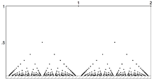
Using Thomae's function f,

${\displaystyle \gcd(a,b)=af\left({\frac {b}{a}}\right),}$

which generalizes to a and b rational numbers or commensurable real numbers.

Keith Slavin has shown that for odd a ≥ 1:

${\displaystyle \gcd(a,b)=\log _{2}\prod _{k=0}^{a-1}(1+e^{-2i\pi kb/a})}$

which is a function that can be evaluated for complex b.[10] Wolfgang Schramm has shown that

${\displaystyle \gcd(a,b)=\sum \limits _{k=1}^{a}\exp(2\pi ikb/a)\cdot \sum \limits _{d\left|a\right.}{\frac {c_{d}(k)}{d}}}$

is an entire function in the variable b for all positive integers a where c_d(k) is Ramanujan's sum.[11]

The computational complexity of the computation of greatest common divisors has been widely studied.[12] If one uses the Euclidean algorithm and the elementary algorithms for multiplication and division, the computation of the greatest common divisor of two integers of at most n bits is ${\displaystyle O(n^{2}).}$ This means that the computation of greatest common divisor has, up to a constant factor, the same complexity as the multiplication.

However, if a fast multiplication algorithm is used, one may modify the Euclidean algorithm for improving the complexity, but the computation of a greatest common divisor becomes slower than the multiplication. More precisely, if the multiplication of two integers of n bits takes a time of T(n), then the fastest known algorithm for greatest common divisor has a complexity ${\displaystyle O\left(T(n)\log n\right).}$ This implies that the fastest known algorithm has a complexity of ${\displaystyle O\left(n\,(\log n)^{2}\log \log n\right).}$

Previous complexities are valid for the usual models of computation, specifically multitape Turing machines and random-access machines.

The computation of the greatest common divisors belongs thus to the class of problems solvable in quasilinear time. A fortiori, the corresponding decision problem belongs to the class P of problems solvable in polynomial time. The GCD problem is not known to be in NC, and so there is no known way to parallelize it efficiently; nor is it known to be P-complete, which would imply that it is unlikely to be possible to efficiently parallelize GCD computation. Shallcross et al. showed that a related problem (EUGCD, determining the remainder sequence arising during the Euclidean algorithm) is NC-equivalent to the problem of integer linear programming with two variables; if either problem is in NC or is P-complete, the other is as well.[13] Since NC contains NL, it is also unknown whether a space-efficient algorithm for computing the GCD exists, even for nondeterministic Turing machines.

Although the problem is not known to be in NC, parallel algorithms asymptotically faster than the Euclidean algorithm exist; the fastest known deterministic algorithm is by Chor and Goldreich, which (in the CRCW-PRAM model) can solve the problem in O(n/log n) time with n^1+ε processors.[14] Randomized algorithms can solve the problem in O((log n)²) time on ${\displaystyle \exp \left(O\left({\sqrt {n\log n}}\right)\right)}$ processors (this is superpolynomial).[15]

References

- Andrews, George E. (1994) [1971], Number Theory, Dover, ISBN 9780486682525
- Hardy, G. H.; Wright, E. M. (1979), An Introduction to the Theory of Numbers (Fifth ed.), Oxford: Oxford University Press, ISBN 978-0-19-853171-5
- Long, Calvin T. (1972), Elementary Introduction to Number Theory (2nd ed.), Lexington: D. C. Heath and Company, LCCN 77171950
- Pettofrezzo, Anthony J.; Byrkit, Donald R. (1970), Elements of Number Theory, Englewood Cliffs: Prentice Hall, LCCN 71081766
Further reading
- Donald Knuth. The Art of Computer Programming, Volume 2: Seminumerical Algorithms, Third Edition. Addison-Wesley, 1997. ISBN 0-201-89684-2. Section 4.5.2: The Greatest Common Divisor, pp. 333–356.
- Thomas H. Cormen, Charles E. Leiserson, Ronald L. Rivest, and Clifford Stein. Introduction to Algorithms, Second Edition. MIT Press and McGraw-Hill, 2001. ISBN 0-262-03293-7. Section 31.2: Greatest common divisor, pp. 856–862.
- Saunders MacLane and Garrett Birkhoff. A Survey of Modern Algebra, Fourth Edition. MacMillan Publishing Co., 1977. ISBN 0-02-310070-2. 1–7: "The Euclidean Algorithm."
External links
- Greatest Common Measure: The Last 2500 Years, by Alexander Stepanov