Least common multiple
In arithmetic and number theory, the least common multiple, lowest common multiple, or smallest common multiple of two integers a and b, usually denoted by LCM(a, b), is the smallest positive integer that is divisible by both a and b.[1] Since division of integers by zero is undefined, this definition has meaning only if a and b are both different from zero.[2] However, some authors define LCM (a,0) as 0 for all a, which is the result of taking the LCM to be the least upper bound in the lattice of divisibility.
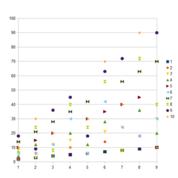
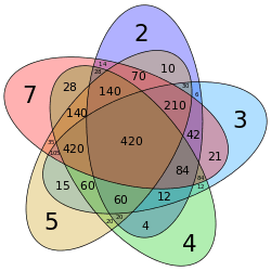
For example, a card game which requires its cards to be divided equally among up to 5 players requires at least 60 cards, the number at the intersection of the 2, 3, 4, and 5 sets, but not the 7 set.
The LCM is the "lowest common denominator" (LCD) that can be used before fractions can be added, subtracted or compared. The LCM of more than two integers is also well-defined: it is the smallest positive integer that is divisible by each of them.
Overview
A multiple of a number is the product of that number and an integer. For example, 10 is a multiple of 5 because 5 × 2 = 10, so 10 is divisible by 5 and 2. Because 10 is the smallest positive integer that is divisible by both 5 and 2, it is the least common multiple of 5 and 2. By the same principle, 10 is the least common multiple of −5 and −2 as well.
Notation
The least common multiple of two integers a and b is denoted as lcm(a, b). Some older textbooks use [a, b],[2][3] while the programming language J uses a*.b .
Example
LCM(4, 6)
Multiples of 4 are:
- 4, 8, 12, 16, 20, 24, 28, 32, 36, 40, 44, 48, 52, 56, 60, 64, 68, 72, 76, ...
Multiples of 6 are:
- 6, 12, 18, 24, 30, 36, 42, 48, 54, 60, 66, 72, ...
Common multiples of 4 and 6 are the numbers that are in both lists:
- 12, 24, 36, 48, 60, 72, ....
So, from this list of the first few common multiples of the numbers 4 and 6, their least common multiple is 12.
Applications
When adding, subtracting, or comparing simple fractions, the least common multiple of the denominators often called the lowest common denominator is used because each of the fractions can be expressed as a fraction with this denominator. For example,

where the denominator 42 was used because it is the least common multiple of 21 and 6.
Gears problem
Suppose there are two meshing gears in a machine, having m and n teeth, respectively, and the gears are marked by a line segment drawn from the center of the first gear to the center of the second gear. When the gears begin rotating, the number of rotations the first gear must complete to realign the line segment can be calculated by using . The first gear must complete rotations for the realignment. By that time, the second gear will have made rotations.


Planetary alignment
Suppose there are three planets revolving around a star which take l, m and n units of time respectively to complete their orbits. Assume that l, m and n are integers. Assuming the planets started moving around the star after an initial linear alignment, all the planets attain a linear alignment again after units of time. At this time, the first, second and third planet will have completed , and orbits respectively around the star.[4]


Calculation
Using the greatest common divisor
The following formula reduces the problem of computing the least common multiple to the problem of computing the greatest common divisor (GCD), also known as the greatest common factor:

This formula is also valid when exactly one of a and b is 0, since gcd(a, 0) = |a|. However, if both a and b are 0, this formula would cause division by zero; lcm(0, 0) = 0 is a special case.
There are fast algorithms for computing the GCD that do not require the numbers to be factored, such as the Euclidean algorithm. To return to the example above,

Because gcd(a, b) is a divisor of both a and b, it is more efficient to compute the LCM by dividing before multiplying:

This reduces the size of one input for both the division and the multiplication, and reduces the required storage needed for intermediate results (overflow in the a×b computation). Because gcd(a, b) is a divisor of both a and b, the division is guaranteed to yield an integer, so the intermediate result can be stored in an integer. Done this way, the previous example becomes:

Using prime factorization
The unique factorization theorem indicates that every positive integer greater than 1 can be written in only one way as a product of prime numbers. The prime numbers can be considered as the atomic elements which, when combined together, make up a composite number.
For example:

Here the composite number 90 is made up of one atom of the prime number 2, two atoms of the prime number 3 and one atom of the prime number 5.
This fact can be used to find the LCM of a set of numbers.
Example: lcm(8,9,21)
Factor each number and express it as a product of prime number powers.

The lcm will be the product of multiplying the highest power of each prime number together. The highest power of the three prime numbers 2, 3, and 7 is 23, 32, and 71, respectively. Thus,

This method is not as efficient as reducing to the greatest common divisor, since there is no known general efficient algorithm for integer factorization.
This method can be illustrated with a Venn diagram as follows with the prime factorization of each of the two numbers demonstrated in each circle and all factors they share in common in the intersection. The LCM can be found by multiplying all of the prime numbers in the diagram.
Here is an example:
- 48 = 2 × 2 × 2 × 2 × 3,
- 180 = 2 × 2 × 3 × 3 × 5,
sharing two "2"s and a "3" in common:

- Least common multiple = 2 × 2 × 2 × 2 × 3 × 3 × 5 = 720
- Greatest common divisor = 2 × 2 × 3 = 12
This also works for the greatest common divisor (GCD), except that instead of multiplying all of the numbers in the Venn diagram, one multiplies only the prime factors that are in the intersection. Thus the GCD of 48 and 180 is 2 × 2 × 3 = 12.
Using a simple algorithm
This method works easily for finding the LCM of several integers.
Let there be a finite sequence of positive integers X = (x1, x2, ..., xn), n > 1. The algorithm proceeds in steps as follows: on each step m it examines and updates the sequence X(m) = (x1(m), x2(m), ..., xn(m)), X(1) = X, where X(m) is the mth iteration of X, that is, X at step m of the algorithm, etc. The purpose of the examination is to pick the least (perhaps, one of many) element of the sequence X(m). Assuming xk0(m) is the selected element, the sequence X(m+1) is defined as
- xk(m+1) = xk(m), k ≠ k0
- xk0(m+1) = xk0(m) + xk0(1).
In other words, the least element is increased by the corresponding x whereas the rest of the elements pass from X(m) to X(m+1) unchanged.
The algorithm stops when all elements in sequence X(m) are equal. Their common value L is exactly LCM(X).
For example, if X = X(1) = (3, 4, 6), the steps in the algorithm produce:
- X(2) = (6, 4, 6)
- X(3) = (6, 8, 6)
- X(4) = (6, 8, 12) - by choosing the second 6
- X(5) = (9, 8, 12)
- X(6) = (9, 12, 12)
- X(7) = (12, 12, 12) so LCM = 12.
Using the table-method
This method works for any number of numbers. One begins by listing all of the numbers vertically in a table (in this example 4, 7, 12, 21, and 42):
- 4
- 7
- 12
- 21
- 42
The process begins by dividing all of the numbers by 2. If 2 divides any of them evenly, write 2 in a new column at the top of the table and the result of division by 2 of each number in the space to the right in this new column. If a number is not evenly divisible, just rewrite the number again. If 2 does not divide evenly into any of the numbers, repeat this procedure with the next largest prime number, 3 (see below).
| x | 2 |
|---|---|
| 4 | 2 |
| 7 | 7 |
| 12 | 6 |
| 21 | 21 |
| 42 | 21 |
Now, assuming that 2 did divide at least one number (as in this example), check if 2 divides again:
| x | 2 | 2 |
|---|---|---|
| 4 | 2 | 1 |
| 7 | 7 | 7 |
| 12 | 6 | 3 |
| 21 | 21 | 21 |
| 42 | 21 | 21 |
Once 2 no longer divides any number in the current column, repeat the procedure by dividing by the next larger prime, 3. Once 3 no longer divides, try the next larger primes, 5 then 7, etc. The process ends when all of the numbers have been reduced to 1 (the column under the last prime divisor consists only of 1's).
| x | 2 | 2 | 3 | 7 |
|---|---|---|---|---|
| 4 | 2 | 1 | 1 | 1 |
| 7 | 7 | 7 | 7 | 1 |
| 12 | 6 | 3 | 1 | 1 |
| 21 | 21 | 21 | 7 | 1 |
| 42 | 21 | 21 | 7 | 1 |
Now, multiply the numbers in the top row to obtain the LCM. In this case, it is 2 × 2 × 3 × 7 = 84.
As a general computational algorithm, the above is quite inefficient. One would never want to implement it in software: it takes too many steps, and requires too much storage space. A far more efficient numerical algorithm can be obtained by using Euclid's algorithm to compute the gcd first, and then obtaining the lcm by division.
Formulas
Fundamental theorem of arithmetic
According to the fundamental theorem of arithmetic a positive integer is the product of prime numbers, and, except for their order, this representation is unique:

where the exponents n2, n3, ... are non-negative integers; for example, 84 = 22 31 50 71 110 130 ...
Given two positive integers and their least common multiple and greatest common divisor are given by the formulas


and

Since

this gives

In fact, every rational number can be written uniquely as the product of primes if negative exponents are allowed. When this is done, the above formulas remain valid. For example:

Lattice-theoretic
The positive integers may be partially ordered by divisibility: if a divides b (that is, if b is an integer multiple of a) write a ≤ b (or equivalently, b ≥ a). (Forget the usual magnitude-based definition of ≤ in this section - it is not used.)
Under this ordering, the positive integers become a lattice with meet given by the gcd and join given by the lcm. The proof is straightforward, if a bit tedious; it amounts to checking that lcm and gcd satisfy the axioms for meet and join. Putting the lcm and gcd into this more general context establishes a duality between them:
- If a formula involving integer variables, gcd, lcm, ≤ and ≥ is true, then the formula obtained by switching gcd with lcm and switching ≥ with ≤ is also true. (Remember ≤ is defined as divides).
The following pairs of dual formulas are special cases of general lattice-theoretic identities.
|


|


It can also be shown[5] that this lattice is distributive; that is, lcm distributes over gcd and gcd distributes over lcm:


This identity is self-dual:


In commutative rings
The least common multiple can be defined generally over commutative rings as follows: Let a and b be elements of a commutative ring R. A common multiple of a and b is an element m of R such that both a and b divide m (that is, there exist elements x and y of R such that ax = m and by = m). A least common multiple of a and b is a common multiple that is minimal in the sense that for any other common multiple n of a and b, m divides n.
In general, two elements in a commutative ring can have no least common multiple or more than one. However, any two least common multiples of the same pair of elements are associates. In a unique factorization domain, any two elements have a least common multiple. In a principal ideal domain, the least common multiple of a and b can be characterised as a generator of the intersection of the ideals generated by a and b (the intersection of a collection of ideals is always an ideal).
See also
- Anomalous cancellation
- Chebyshev function
Notes
- Hardy & Wright, § 5.1, p. 48
- Long (1972, p. 39)
- Pettofrezzo & Byrkit (1970, p. 56)
- "nasa spacemath" (PDF).
- The next three formulas are from Landau, Ex. III.3, p. 254
- Crandall & Pomerance, ex. 2.4, p. 101.
- Long (1972, p. 41)
- Pettofrezzo & Byrkit (1970, p. 58)
References
- Crandall, Richard; Pomerance, Carl (2001), Prime Numbers: A Computational Perspective, New York: Springer, ISBN 0-387-94777-9
- Hardy, G. H.; Wright, E. M. (1979), An Introduction to the Theory of Numbers (Fifth edition), Oxford: Oxford University Press, ISBN 978-0-19-853171-5
- Landau, Edmund (1966), Elementary Number Theory, New York: Chelsea
- Long, Calvin T. (1972), Elementary Introduction to Number Theory (2nd ed.), Lexington: D. C. Heath and Company, LCCN 77-171950
- Pettofrezzo, Anthony J.; Byrkit, Donald R. (1970), Elements of Number Theory, Englewood Cliffs: Prentice Hall, LCCN 77-81766
| Division and ratio | |||
|---|---|---|---|
| Fraction |
| ||
| |||