Uncertainty quantification

Uncertainty is sometimes classified into two categories,[5][6] prominently seen in medical applications.[7]

Aleatoric uncertainty

Aleatoric uncertainty is also known as statistical uncertainty, and is representative of unknowns that differ each time we run the same experiment. For example, a single arrow shot with a mechanical bow that exactly duplicates each launch (the same acceleration, altitude, direction and final velocity) will not all impact the same point on the target due to random and complicated vibrations of the arrow shaft, the knowledge of which cannot be determined sufficiently to eliminate the resulting scatter of impact points. The argument here is obviously in the definition of "cannot". Just because we cannot measure sufficiently with our currently available measurement devices does not preclude necessarily the existence of such information, which would move this uncertainty into the below category. Aleatoric is derived from the Latin alea or dice, referring to a game of chance.

Epistemic uncertainty

Epistemic uncertainty is also known as systematic uncertainty, and is due to things one could in principle know but do not in practice. This may be because a measurement is not accurate, because the model neglects certain effects, or because particular data has been deliberately hidden. An example of a source of this uncertainty would be the drag in an experiment designed to measure the acceleration of gravity near the earth's surface. The commonly used gravitational acceleration of 9.8 m/s^2 ignores the effects of air resistance, but the air resistance for the object could be measured and incorporated into the experiment to reduce the resulting uncertainty in the calculation of the gravitational acceleration.

In real life applications, both kinds of uncertainties are present. Uncertainty quantification intends to work toward reducing epistemic uncertainties to aleatoric uncertainties. The quantification for the aleatoric uncertainties can be relatively straightforward to perform, depending on the application. Techniques such as the Monte Carlo method are frequently used. A probability distribution can be represented by its moments (in the Gaussian case, the mean and covariance suffice, although, in general, even knowledge of all moments to arbitrarily high order still does not specify the distribution function uniquely), or more recently, by techniques such as Karhunen–Loève and polynomial chaos expansions. To evaluate epistemic uncertainties, the efforts are made to gain better knowledge of the system, process or mechanism. Methods such as probability bounds analysis, fuzzy logic or evidence theory (Dempster–Shafer theory – a generalization of the Bayesian theory of subjective probability) are used.

Uncertainty propagation is the quantification of uncertainties in system output(s) propagated from uncertain inputs. It focuses on the influence on the outputs from the parametric variability listed in the sources of uncertainty. The targets of uncertainty propagation analysis can be:

• To evaluate low-order moments of the outputs, i.e. mean and variance.
• To evaluate the reliability of the outputs. This is especially useful in reliability engineering where outputs of a system are usually closely related to the performance of the system.
• To assess the complete probability distribution of the outputs. This is useful in the scenario of utility optimization where the complete distribution is used to calculate the utility.

Given some experimental measurements of a system and some computer simulation results from its mathematical model, inverse uncertainty quantification estimates the discrepancy between the experiment and the mathematical model (which is called bias correction), and estimates the values of unknown parameters in the model if there are any (which is called parameter calibration or simply calibration). Generally this is a much more difficult problem than forward uncertainty propagation; however it is of great importance since it is typically implemented in a model updating process. There are several scenarios in inverse uncertainty quantification:

The outcome of bias correction, including an updated model (prediction mean) and prediction confidence interval.

Bias correction quantifies the model inadequacy, i.e. the discrepancy between the experiment and the mathematical model. The general model updating formula for bias correction is:

${\displaystyle y^{e}(\mathbf {x} )=y^{m}(\mathbf {x} )+\delta (\mathbf {x} )+\varepsilon }$

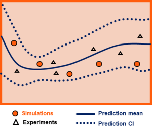
where ${\displaystyle y^{e}(\mathbf {x} )}$ denotes the experimental measurements as a function of several input variables ${\displaystyle \mathbf {x} }$, ${\displaystyle y^{m}(\mathbf {x} )}$ denotes the computer model (mathematical model) response, ${\displaystyle \delta (\mathbf {x} )}$ denotes the additive discrepancy function (aka bias function), and ${\displaystyle \varepsilon }$ denotes the experimental uncertainty. The objective is to estimate the discrepancy function ${\displaystyle \delta (\mathbf {x} )}$, and as a by-product, the resulting updated model is ${\displaystyle y^{m}(\mathbf {x} )+\delta (\mathbf {x} )}$. A prediction confidence interval is provided with the updated model as the quantification of the uncertainty.

Parameter calibration estimates the values of one or more unknown parameters in a mathematical model. The general model updating formulation for calibration is:

${\displaystyle y^{e}(\mathbf {x} )=y^{m}(\mathbf {x} ,{\boldsymbol {\theta }}^{*})+\varepsilon }$

where ${\displaystyle y^{m}(\mathbf {x} ,{\boldsymbol {\theta }})}$ denotes the computer model response that depends on several unknown model parameters ${\displaystyle {\boldsymbol {\theta }}}$, and ${\displaystyle {\boldsymbol {\theta }}^{*}}$ denotes the true values of the unknown parameters in the course of experiments. The objective is to either estimate ${\displaystyle {\boldsymbol {\theta }}^{*}}$, or to come up with a probability distribution of ${\displaystyle {\boldsymbol {\theta }}^{*}}$ that encompasses the best knowledge of the true parameter values.

It considers an inaccurate model with one or more unknown parameters, and its model updating formulation combines the two together:

${\displaystyle y^{e}(\mathbf {x} )=y^{m}(\mathbf {x} ,{\boldsymbol {\theta }}^{*})+\delta (\mathbf {x} )+\varepsilon }$

It is the most comprehensive model updating formulation that includes all possible sources of uncertainty, and it requires the most effort to solve.

Existing uncertainty propagation approaches include probabilistic approaches and non-probabilistic approaches. There are basically five categories of probabilistic approaches for uncertainty propagation:[8]

• Simulation-based methods: Monte Carlo simulations, importance sampling, adaptive sampling, etc.
• Local expansion-based methods: Taylor series, perturbation method, etc. These methods have advantages when dealing with relatively small input variability and outputs that don't express high nonlinearity. These linear or linearized methods are detailed in the article Uncertainty propagation.
• Functional expansion-based methods: Neumann expansion, orthogonal or Karhunen–Loeve expansions (KLE), with polynomial chaos expansion (PCE) and wavelet expansions as special cases.
• Most probable point (MPP)-based methods: first-order reliability method (FORM) and second-order reliability method (SORM).
• Numerical integration-based methods: Full factorial numerical integration (FFNI) and dimension reduction (DR).

For non-probabilistic approaches, interval analysis,[9] Fuzzy theory, possibility theory and evidence theory are among the most widely used.

The probabilistic approach is considered as the most rigorous approach to uncertainty analysis in engineering design due to its consistency with the theory of decision analysis. Its cornerstone is the calculation of probability density functions for sampling statistics.[10] This can be performed rigorously for random variables that are obtainable as transformations of Gaussian variables, leading to exact confidence intervals.

In regression analysis and least squares problems, the standard error of parameter estimates is readily available, which can be expanded into a confidence interval.

Several methodologies for inverse uncertainty quantification exist under the Bayesian framework. The most complicated direction is to aim at solving problems with both bias correction and parameter calibration. The challenges of such problems include not only the influences from model inadequacy and parameter uncertainty, but also the lack of data from both computer simulations and experiments. A common situation is that the input settings are not the same over experiments and simulations.

An approach to inverse uncertainty quantification is the modular Bayesian approach.[4][11] The modular Bayesian approach derives its name from its four-module procedure. Apart from the current available data, a prior distribution of unknown parameters should be assigned.

Module 1: Gaussian process modeling for the computer model

To address the issue from lack of simulation results, the computer model is replaced with a Gaussian process (GP) model

${\displaystyle y^{m}(\mathbf {x} ,{\boldsymbol {\theta }})\sim {\mathcal {GP}}{\big (}\mathbf {h} ^{m}(\cdot )^{T}{\boldsymbol {\beta }}^{m},\sigma _{m}^{2}R^{m}(\cdot ,\cdot ){\big )}}$

where

${\displaystyle R^{m}{\big (}(\mathbf {x} ,{\boldsymbol {\theta }}),(\mathbf {x} ',{\boldsymbol {\theta }}'){\big )}=\exp \left\{-\sum _{k=1}^{d}\omega _{k}^{m}(x_{k}-x_{k}')^{2}\right\}\exp \left\{-\sum _{k=1}^{r}\omega _{d+k}^{m}(\theta _{k}-\theta _{k}')^{2}\right\}.}$

${\displaystyle d}$ is the dimension of input variables, and ${\displaystyle r}$ is the dimension of unknown parameters. While ${\displaystyle \mathbf {h} ^{m}(\cdot )}$ is pre-defined, ${\displaystyle \left\{{\boldsymbol {\beta }}^{m},\sigma _{m},\omega _{k}^{m},k=1,\ldots ,d+r\right\}}$, known as hyperparameters of the GP model, need to be estimated via maximum likelihood estimation (MLE). This module can be considered as a generalized kriging method.

Module 2: Gaussian process modeling for the discrepancy function

Similarly with the first module, the discrepancy function is replaced with a GP model

${\displaystyle \delta (\mathbf {x} )\sim {\mathcal {GP}}{\big (}\mathbf {h} ^{\delta }(\cdot )^{T}{\boldsymbol {\beta }}^{\delta },\sigma _{\delta }^{2}R^{\delta }(\cdot ,\cdot ){\big )}}$

where

${\displaystyle R^{\delta }(\mathbf {x} ,\mathbf {x} ')=\exp \left\{-\sum _{k=1}^{d}\omega _{k}^{\delta }(x_{k}-x_{k}')^{2}\right\}.}$

Together with the prior distribution of unknown parameters, and data from both computer models and experiments, one can derive the maximum likelihood estimates for ${\displaystyle \left\{{\boldsymbol {\beta }}^{\delta },\sigma _{\delta },\omega _{k}^{\delta },k=1,\ldots ,d\right\}}$. At the same time, ${\displaystyle {\boldsymbol {\beta }}^{m}}$ from Module 1 gets updated as well.

Module 3: Posterior distribution of unknown parameters

Bayes' theorem is applied to calculate the posterior distribution of the unknown parameters:

${\displaystyle p({\boldsymbol {\theta }}\mid {\text{data}},{\boldsymbol {\varphi }})\propto p({\rm {{data}\mid {\boldsymbol {\theta }},{\boldsymbol {\varphi }})p({\boldsymbol {\theta }})}}}$

where ${\displaystyle {\boldsymbol {\varphi }}}$ includes all the fixed hyperparameters in previous modules.

Module 4: Prediction of the experimental response and discrepancy function

Fully Bayesian approach requires that not only the priors for unknown parameters ${\displaystyle {\boldsymbol {\theta }}}$ but also the priors for the other hyperparameters ${\displaystyle {\boldsymbol {\varphi }}}$ should be assigned. It follows the following steps:[12]

1. Derive the posterior distribution ${\displaystyle p({\boldsymbol {\theta }},{\boldsymbol {\varphi }}\mid {\text{data}})}$;
2. Integrate ${\displaystyle {\boldsymbol {\varphi }}}$ out and obtain ${\displaystyle p({\boldsymbol {\theta }}\mid {\text{data}})}$. This single step accomplishes the calibration;
3. Prediction of the experimental response and discrepancy function.

However, the approach has significant drawbacks:

• For most cases, ${\displaystyle p({\boldsymbol {\theta }},{\boldsymbol {\varphi }}\mid {\text{data}})}$ is a highly intractable function of ${\displaystyle {\boldsymbol {\varphi }}}$. Hence the integration becomes very troublesome. Moreover, if priors for the other hyperparameters ${\displaystyle {\boldsymbol {\varphi }}}$ are not carefully chosen, the complexity in numerical integration increases even more.
• In the prediction stage, the prediction (which should at least include the expected value of system responses) also requires numerical integration. Markov chain Monte Carlo (MCMC) is often used for integration; however it is computationally expensive.

The fully Bayesian approach requires a huge amount of calculations and may not yet be practical for dealing with the most complicated modelling situations.[12]

References

- Sacks, Jerome; Welch, William J.; Mitchell, Toby J.; Wynn, Henry P. (1989). "Design and Analysis of Computer Experiments". Statistical Science. 4 (4): 409–423. doi:10.1214/ss/1177012413. JSTOR 2245858.
- Ronald L. Iman, Jon C. Helton, "An Investigation of Uncertainty and Sensitivity Analysis Techniques for Computer Models", Risk Analysis, Volume 8, Issue 1, pages 71–90, March 1988, doi:10.1111/j.1539-6924.1988.tb01155.x
- W.E. Walker, P. Harremoës, J. Rotmans, J.P. van der Sluijs, M.B.A. van Asselt, P. Janssen and M.P. Krayer von Krauss, "Defining Uncertainty: A Conceptual Basis for Uncertainty Management in Model-Based Decision Support", Integrated Assessment, Volume 4, Issue 1, 2003, doi:10.1076/iaij.4.1.5.16466
- Kennedy, Marc C.; O'Hagan, Anthony (2001). "Bayesian calibration of computer models". Journal of the Royal Statistical Society: Series B (Statistical Methodology). 63 (3): 425–464. doi:10.1111/1467-9868.00294.
- Der Kiureghian, Armen; Ditlevsen, Ove (2009). "Aleatory or epistemic? Does it matter?". Structural Safety. 31 (2): 105–112. doi:10.1016/j.strusafe.2008.06.020.
- Matthies, Hermann G. (2007). "Quantifying Uncertainty: Modern Computational Representation of Probability and Applications". Extreme Man-Made and Natural Hazards in Dynamics of Structures. NATO Security through Science Series. pp. 105–135. doi:10.1007/978-1-4020-5656-7_4. ISBN 978-1-4020-5654-3.
- Abhaya Indrayan, Medical Biostatistics, Second Edition, Chapman & Hall/CRC Press, 2008, pages 8, 673
- S. H. Lee and W. Chen, "A comparative study of uncertainty propagation methods for black-box-type problems", Structural and Multidisciplinary Optimization Volume 37, Number 3 (2009), 239–253, doi:10.1007/s00158-008-0234-7
- Jaulin, L.; Kieffer, M.; Didrit, O.; Walter, E. (2001). Applied Interval Analysis. Springer. ISBN 1-85233-219-0.
- Arnaut, L. R. Measurement uncertainty in reverberation chambers - I. Sample statistics. Technical report TQE 2, 2nd. ed., sec. 3.1, National Physical Laboratory, 2008.
- Marc C. Kennedy, Anthony O'Hagan, Supplementary Details on Bayesian Calibration of Computer Models, Sheffield, University of Sheffield: 1–13, 2000
- F. Liu, M. J. Bayarri and J.O.Berger, "Modularization in Bayesian Analysis, with Emphasis on Analysis of Computer Models", Bayesian Analysis (2009) 4, Number 1, pp. 119–150, doi:10.1214/09-BA404
- Paul D. Arendt, Daniel W. Apley, Wei Chen, David Lamb and David Gorsich , "Improving Identifiability in Model Calibration Using Multiple Responses", Journal of Mechanical Design, 134(10), 100909 (2012); doi:10.1115/1.4007573