Drag (physics)
In fluid dynamics, drag (sometimes called air resistance, a type of friction, or fluid resistance, another type of friction or fluid friction) is a force acting opposite to the relative motion of any object moving with respect to a surrounding fluid.[1] This can exist between two fluid layers (or surfaces) or a fluid and a solid surface. Unlike other resistive forces, such as dry friction, which are nearly independent of velocity, drag forces depend on velocity.[2][3] Drag force is proportional to the velocity for a laminar flow and the squared velocity for a turbulent flow. Even though the ultimate cause of a drag is viscous friction, the turbulent drag is independent of viscosity.[4]
| Shape and flow | Form Drag |
Skin friction |
|---|---|---|
| 0% | 100% | |
| ~10% | ~90% | |
 |
~90% | ~10% |
 |
100% | 0% |
Drag forces always decrease fluid velocity relative to the solid object in the fluid's path.
Examples of drag
Examples of drag include the component of the net aerodynamic or hydrodynamic force acting opposite to the direction of movement of a solid object such as cars, aircraft[3] and boat hulls; or acting in the same geographical direction of motion as the solid, as for sails attached to a down wind sail boat, or in intermediate directions on a sail depending on points of sail.[5][6][7] In the case of viscous drag of fluid in a pipe, drag force on the immobile pipe decreases fluid velocity relative to the pipe.[8][9]
In the physics of sports, the drag force is necessary to explain the performance of runners, particularly of sprinters.[10]
Types of drag
Types of drag are generally divided into the following categories:
- parasitic drag, consisting of
- lift-induced drag, and
- wave drag (aerodynamics) or wave resistance (ship hydrodynamics).
The phrase parasitic drag is mainly used in aerodynamics, since for lifting wings, drag is generally small compared to lift. For flow around bluff bodies, form drag and skin friction drag dominate, and then the qualifier "parasitic" is meaningless.
- Base drag, (Aerodynamics) drag generated in an object moving through a fluid from the shape of its rear side.
Further, lift-induced drag is only relevant when wings or a lifting body are present, and is therefore usually discussed either in aviation or in the design of semi-planing or planing hulls. Wave drag occurs either when a solid object is moving through a gas at or near the speed of sound or when a solid object is moving along a fluid boundary, as in surface waves.

Drag depends on the properties of the fluid and on the size, shape, and speed of the object. One way to express this is by means of the drag equation:

where
- is the drag force,
- is the density of the fluid,[11]
- is the speed of the object relative to the fluid,
- is the cross sectional area, and
- is the drag coefficient – a dimensionless number.


The drag coefficient depends on the shape of the object and on the Reynolds number
- ,

where is some characteristic diameter or linear dimension and is the kinematic viscosity of the fluid (equal to the viscosity divided by the density ). At low , is asymptotically proportional to , which means that the drag is linearly proportional to the speed. At high , is more or less constant and drag will vary as the square of the speed. The graph to the right shows how varies with for the case of a sphere. Since the power needed to overcome the drag force is the product of the force times speed, the power needed to overcome drag will vary as the square of the speed at low Reynolds numbers and as the cube of the speed at high numbers.


It can be demonstrated that drag force can be expressed as a function of a dimensionless number, which is dimensionally identical to the Bejan number.[12] Consequently, drag force and drag coefficient can be a function of Bejan number. In fact, from the expression of drag force it has been obtained:

and consequently allows expressing the drag coefficient as a function of Bejan number and the ratio between wet area and front area :[12]


where is the Reynold Number related to fluid path length L.

Drag at high velocity
As mentioned, the drag equation with a constant drag coefficient gives the force experienced by an object moving through a fluid at relatively large velocity (i.e. high Reynolds number, Re > ~1000). This is also called quadratic drag. The equation is attributed to Lord Rayleigh, who originally used L2 in place of A (L being some length).

The reference area A is often orthographic projection of the object (frontal area)—on a plane perpendicular to the direction of motion—e.g. for objects with a simple shape, such as a sphere, this is the cross sectional area. Sometimes a body is a composite of different parts, each with a different reference areas, in which case a drag coefficient corresponding to each of those different areas must be determined.
In the case of a wing the reference areas are the same and the drag force is in the same ratio to the lift force as the ratio of drag coefficient to lift coefficient.[13] Therefore, the reference for a wing is often the lifting area ("wing area") rather than the frontal area.[14]
For an object with a smooth surface, and non-fixed separation points—like a sphere or circular cylinder—the drag coefficient may vary with Reynolds number Re, even up to very high values (Re of the order 107). [15] [16] For an object with well-defined fixed separation points, like a circular disk with its plane normal to the flow direction, the drag coefficient is constant for Re > 3,500.[16] Further the drag coefficient Cd is, in general, a function of the orientation of the flow with respect to the object (apart from symmetrical objects like a sphere).
Power
Under the assumption that the fluid is not moving relative to the currently used reference system, the power required to overcome the aerodynamic drag is given by:

Note that the power needed to push an object through a fluid increases as the cube of the velocity. A car cruising on a highway at 50 mph (80 km/h) may require only 10 horsepower (7.5 kW) to overcome aerodynamic drag, but that same car at 100 mph (160 km/h) requires 80 hp (60 kW).[17] With a doubling of speed the drag (force) quadruples per the formula. Exerting 4 times the force over a fixed distance produces 4 times as much work. At twice the speed the work (resulting in displacement over a fixed distance) is done twice as fast. Since power is the rate of doing work, 4 times the work done in half the time requires 8 times the power.
When the fluid is moving relative to the reference system (e.g. a car driving into headwind) the power required to overcome the aerodynamic drag is given by:

Where is the wind speed and is the object speed (both relative to ground).


Velocity of a falling object
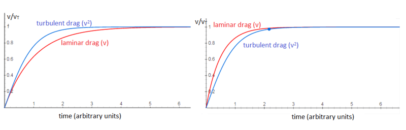
The velocity as a function of time for an object falling through a non-dense medium, and released at zero relative-velocity v = 0 at time t = 0, is roughly given by a function involving a hyperbolic tangent (tanh):

The hyperbolic tangent has a limit value of one, for large time t. In other words, velocity asymptotically approaches a maximum value called the terminal velocity vt:

For an object falling and released at relative-velocity v = vi at time t = 0, with vi ≤ vt, is also defined in terms of the hyperbolic tangent function:

Actually, this function is defined by the solution of the following differential equation:

Or, more generically (where F(v) are the forces acting on the object beyond drag):

For a potato-shaped object of average diameter d and of density ρobj, terminal velocity is about

For objects of water-like density (raindrops, hail, live objects—mammals, birds, insects, etc.) falling in air near Earth's surface at sea level, the terminal velocity is roughly equal to

with d in metre and vt in m/s. For example, for a human body ( ~ 0.6 m) ~ 70 m/s, for a small animal like a cat ( ~ 0.2 m) ~ 40 m/s, for a small bird ( ~ 0.05 m) ~ 20 m/s, for an insect ( ~ 0.01 m) ~ 9 m/s, and so on. Terminal velocity for very small objects (pollen, etc.) at low Reynolds numbers is determined by Stokes law.


Terminal velocity is higher for larger creatures, and thus potentially more deadly. A creature such as a mouse falling at its terminal velocity is much more likely to survive impact with the ground than a human falling at its terminal velocity. A small animal such as a cricket impacting at its terminal velocity will probably be unharmed. This, combined with the relative ratio of limb cross-sectional area vs. body mass (commonly referred to as the Square-cube law), explains why very small animals can fall from a large height and not be harmed.[18]
Very low Reynolds numbers: Stokes' drag
The equation for viscous resistance or linear drag is appropriate for objects or particles moving through a fluid at relatively slow speeds where there is no turbulence (i.e. low Reynolds number, ).[19] Note that purely laminar flow only exists up to Re = 0.1 under this definition. In this case, the force of drag is approximately proportional to velocity. The equation for viscous resistance is:[20]


where:
- is a constant that depends on the properties of the fluid and the dimensions of the object, and
- is the velocity of the object


When an object falls from rest, its velocity will be

which asymptotically approaches the terminal velocity . For a given , heavier objects fall more quickly.

For the special case of small spherical objects moving slowly through a viscous fluid (and thus at small Reynolds number), George Gabriel Stokes derived an expression for the drag constant:

where:
- is the Stokes radius of the particle, and is the fluid viscosity.


The resulting expression for the drag is known as Stokes' drag:[21]

For example, consider a small sphere with radius = 0.5 micrometre (diameter = 1.0 µm) moving through water at a velocity of 10 µm/s. Using 10−3 Pa·s as the dynamic viscosity of water in SI units, we find a drag force of 0.09 pN. This is about the drag force that a bacterium experiences as it swims through water.

The drag coefficient of a sphere can be determined for the general case of a laminar flow with Reynolds numbers less than 1 using the following formula[22]:


For Reynolds numbers less than 1, Stokes' law applies and the drag coefficient approaches !

Aerodynamics
In aerodynamics, aerodynamic drag is the fluid drag force that acts on any moving solid body in the direction of the fluid freestream flow.[23] From the body's perspective (near-field approach), the drag results from forces due to pressure distributions over the body surface, symbolized , and forces due to skin friction, which is a result of viscosity, denoted . Alternatively, calculated from the flowfield perspective (far-field approach), the drag force results from three natural phenomena: shock waves, vortex sheet, and viscosity.


Overview
The pressure distribution acting on a body's surface exerts normal forces on the body. Those forces can be summed and the component of that force that acts downstream represents the drag force, , due to pressure distribution acting on the body. The nature of these normal forces combines shock wave effects, vortex system generation effects, and wake viscous mechanisms.
The viscosity of the fluid has a major effect on drag. In the absence of viscosity, the pressure forces acting to retard the vehicle are canceled by a pressure force further aft that acts to push the vehicle forward; this is called pressure recovery and the result is that the drag is zero. That is to say, the work the body does on the airflow, is reversible and is recovered as there are no frictional effects to convert the flow energy into heat. Pressure recovery acts even in the case of viscous flow. Viscosity, however results in pressure drag and it is the dominant component of drag in the case of vehicles with regions of separated flow, in which the pressure recovery is fairly ineffective.
The friction drag force, which is a tangential force on the aircraft surface, depends substantially on boundary layer configuration and viscosity. The net friction drag, , is calculated as the downstream projection of the viscous forces evaluated over the body's surface.
The sum of friction drag and pressure (form) drag is called viscous drag. This drag component is due to viscosity. In a thermodynamic perspective, viscous effects represent irreversible phenomena and, therefore, they create entropy. The calculated viscous drag use entropy changes to accurately predict the drag force.

When the airplane produces lift, another drag component results. Induced drag, symbolized , is due to a modification of the pressure distribution due to the trailing vortex system that accompanies the lift production. An alternative perspective on lift and drag is gained from considering the change of momentum of the airflow. The wing intercepts the airflow and forces the flow to move downward. This results in an equal and opposite force acting upward on the wing which is the lift force. The change of momentum of the airflow downward results in a reduction of the rearward momentum of the flow which is the result of a force acting forward on the airflow and applied by the wing to the air flow; an equal but opposite force acts on the wing rearward which is the induced drag. Induced drag tends to be the most important component for airplanes during take-off or landing flight. Another drag component, namely wave drag, , results from shock waves in transonic and supersonic flight speeds. The shock waves induce changes in the boundary layer and pressure distribution over the body surface.


History
The idea that a moving body passing through air or another fluid encounters resistance had been known since the time of Aristotle. Louis Charles Breguet's paper of 1922 began efforts to reduce drag by streamlining.[24] Breguet went on to put his ideas into practice by designing several record-breaking aircraft in the 1920s and 1930s. Ludwig Prandtl's boundary layer theory in the 1920s provided the impetus to minimise skin friction. A further major call for streamlining was made by Sir Melvill Jones who provided the theoretical concepts to demonstrate emphatically the importance of streamlining in aircraft design.[25][26][27] In 1929 his paper ‘The Streamline Airplane’ presented to the Royal Aeronautical Society was seminal. He proposed an ideal aircraft that would have minimal drag which led to the concepts of a 'clean' monoplane and retractable undercarriage. The aspect of Jones's paper that most shocked the designers of the time was his plot of the horse power required versus velocity, for an actual and an ideal plane. By looking at a data point for a given aircraft and extrapolating it horizontally to the ideal curve, the velocity gain for the same power can be seen. When Jones finished his presentation, a member of the audience described the results as being of the same level of importance as the Carnot cycle in thermodynamics.[24][25]
Lift-induced drag
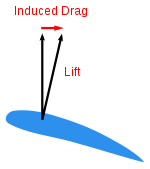
Lift-induced drag (also called induced drag) is drag which occurs as the result of the creation of lift on a three-dimensional lifting body, such as the wing or fuselage of an airplane. Induced drag consists primarily of two components: drag due to the creation of trailing vortices (vortex drag); and the presence of additional viscous drag (lift-induced viscous drag) that is not present when lift is zero. The trailing vortices in the flow-field, present in the wake of a lifting body, derive from the turbulent mixing of air from above and below the body which flows in slightly different directions as a consequence of creation of lift.
With other parameters remaining the same, as the lift generated by a body increases, so does the lift-induced drag. This means that as the wing's angle of attack increases (up to a maximum called the stalling angle), the lift coefficient also increases, and so too does the lift-induced drag. At the onset of stall, lift is abruptly decreased, as is lift-induced drag, but viscous pressure drag, a component of parasite drag, increases due to the formation of turbulent unattached flow in the wake behind the body.
Parasitic drag
Parasitic drag is drag caused by moving a solid object through a fluid. Parasitic drag is made up of multiple components including viscous pressure drag (form drag), and drag due to surface roughness (skin friction drag). Additionally, the presence of multiple bodies in relative proximity may incur so called interference drag, which is sometimes described as a component of parasitic drag.
In aviation, induced drag tends to be greater at lower speeds because a high angle of attack is required to maintain lift, creating more drag. However, as speed increases the angle of attack can be reduced and the induced drag decreases. Parasitic drag, however, increases because the fluid is flowing more quickly around protruding objects increasing friction or drag. At even higher speeds (transonic), wave drag enters the picture. Each of these forms of drag changes in proportion to the others based on speed. The combined overall drag curve therefore shows a minimum at some airspeed - an aircraft flying at this speed will be at or close to its optimal efficiency. Pilots will use this speed to maximize endurance (minimum fuel consumption), or maximize gliding range in the event of an engine failure.
Power curve in aviation
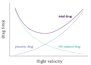
The interaction of parasitic and induced drag vs. airspeed can be plotted as a characteristic curve, illustrated here. In aviation, this is often referred to as the power curve, and is important to pilots because it shows that, below a certain airspeed, maintaining airspeed counterintuitively requires more thrust as speed decreases, rather than less. The consequences of being "behind the curve" in flight are important and are taught as part of pilot training. At the subsonic airspeeds where the "U" shape of this curve is significant, wave drag has not yet become a factor, and so it is not shown in the curve.
Wave drag in transonic and supersonic flow

Wave drag (also called compressibility drag) is drag that is created when a body moves in a compressible fluid and at speeds that are close to the speed of sound in that fluid. In aerodynamics, wave drag consists of multiple components depending on the speed regime of the flight.
In transonic flight (Mach numbers greater than about 0.8 and less than about 1.4), wave drag is the result of the formation of shockwaves in the fluid, formed when local areas of supersonic (Mach number greater than 1.0) flow are created. In practice, supersonic flow occurs on bodies traveling well below the speed of sound, as the local speed of air increases as it accelerates over the body to speeds above Mach 1.0. However, full supersonic flow over the vehicle will not develop until well past Mach 1.0. Aircraft flying at transonic speed often incur wave drag through the normal course of operation. In transonic flight, wave drag is commonly referred to as transonic compressibility drag. Transonic compressibility drag increases significantly as the speed of flight increases towards Mach 1.0, dominating other forms of drag at those speeds.
In supersonic flight (Mach numbers greater than 1.0), wave drag is the result of shockwaves present in the fluid and attached to the body, typically oblique shockwaves formed at the leading and trailing edges of the body. In highly supersonic flows, or in bodies with turning angles sufficiently large, unattached shockwaves, or bow waves will instead form. Additionally, local areas of transonic flow behind the initial shockwave may occur at lower supersonic speeds, and can lead to the development of additional, smaller shockwaves present on the surfaces of other lifting bodies, similar to those found in transonic flows. In supersonic flow regimes, wave drag is commonly separated into two components, supersonic lift-dependent wave drag and supersonic volume-dependent wave drag.
The closed form solution for the minimum wave drag of a body of revolution with a fixed length was found by Sears and Haack, and is known as the Sears-Haack Distribution. Similarly, for a fixed volume, the shape for minimum wave drag is the Von Karman Ogive.
The Busemann biplane is not, in principle, subject to wave drag when operated at its design speed, but is incapable of generating lift in this condition.
d'Alembert's paradox
In 1752 d'Alembert proved that potential flow, the 18th century state-of-the-art inviscid flow theory amenable to mathematical solutions, resulted in the prediction of zero drag. This was in contradiction with experimental evidence, and became known as d'Alembert's paradox. In the 19th century the Navier–Stokes equations for the description of viscous flow were developed by Saint-Venant, Navier and Stokes. Stokes derived the drag around a sphere at very low Reynolds numbers, the result of which is called Stokes' law.[30]
In the limit of high Reynolds numbers, the Navier–Stokes equations approach the inviscid Euler equations, of which the potential-flow solutions considered by d'Alembert are solutions. However, all experiments at high Reynolds numbers showed there is drag. Attempts to construct inviscid steady flow solutions to the Euler equations, other than the potential flow solutions, did not result in realistic results.[30]
The notion of boundary layers—introduced by Prandtl in 1904, founded on both theory and experiments—explained the causes of drag at high Reynolds numbers. The boundary layer is the thin layer of fluid close to the object's boundary, where viscous effects remain important even when the viscosity is very small (or equivalently the Reynolds number is very large).[30]
See also
- Added mass
- Aerodynamic force
- Angle of attack
- Boundary layer
- Coandă effect
- Drag crisis
- Drag coefficient
- Drag equation
- Gravity drag
- Keulegan–Carpenter number
- Lift (force)
- Morison equation
- Nose cone design
- Parasitic drag
- Ram pressure
- Reynolds number
- Stall (fluid mechanics)
- Stokes' law
- Terminal velocity
- Wave drag
- Windage
References
- "Definition of DRAG". www.merriam-webster.com.
- French (1970), p. 211, Eq. 7-20
- "What is Drag?". Archived from the original on 2010-05-24. Retrieved 2011-10-16.
- G. Falkovich (2011). Fluid Mechanics (A short course for physicists). Cambridge University Press. ISBN 978-1-107-00575-4.
- Eiffel, Gustave (1913). The Resistance of The Air and Aviation. London: Constable &Co Ltd.
- Marchaj, C. A. (2003). Sail performance : techniques to maximise sail power (Rev. ed.). London: Adlard Coles Nautical. pp. 147 figure 127 lift vs drag polar curves. ISBN 978-0-7136-6407-2.
- Drayton, Fabio Fossati; translated by Martyn (2009). Aero-hydrodynamics and the performance of sailing yachts : the science behind sailing yachts and their design. Camden, Maine: International Marine /McGraw-Hill. pp. 98 Fig 5.17 Chapter five Sailing Boat Aerodynamics. ISBN 978-0-07-162910-2.
- "Calculating Viscous Flow: Velocity Profiles in Rivers and Pipes" (PDF). Retrieved 16 October 2011.
- "Viscous Drag Forces". Retrieved 16 October 2011.
- Hernandez-Gomez, J J; Marquina, V; Gomez, R W (25 July 2013). "On the performance of Usain Bolt in the 100 m sprint". Eur. J. Phys. 34 (5): 1227. arXiv:1305.3947. Bibcode:2013EJPh...34.1227H. doi:10.1088/0143-0807/34/5/1227. Retrieved 23 April 2016.
- Note that for Earth's atmosphere, the air density can be found using the barometric formula. It is 1.293 kg/m3 at 0 °C and 1 atmosphere.
- Liversage, P., and Trancossi, M. (2018). Analysis of triangular sharkskin profiles according to second law, Modelling, Measurement and Control B. 87(3), 188-196. http://www.iieta.org/sites/default/files/Journals/MMC/MMC_B/87.03_11.pdf
- Size effects on drag Archived 2016-11-09 at the Wayback Machine, from NASA Glenn Research Center.
- Wing geometry definitions Archived 2011-03-07 at the Wayback Machine, from NASA Glenn Research Center.
- Roshko, Anatol (1961). "Experiments on the flow past a circular cylinder at very high Reynolds number" (PDF). Journal of Fluid Mechanics. 10 (3): 345–356. Bibcode:1961JFM....10..345R. doi:10.1017/S0022112061000950.
- Batchelor (1967), p. 341.
- Brian Beckman (1991). "Part 6: Speed and Horsepower". Retrieved 18 May 2016.
- Haldane, J.B.S., "On Being the Right Size"
- Drag Force Archived April 14, 2008, at the Wayback Machine
- Air friction, from Department of Physics and Astronomy, Georgia State University
- Collinson, Chris; Roper, Tom (1995). Particle Mechanics. Butterworth-Heinemann. p. 30. ISBN 9780080928593.
- tec-science (2020-05-31). "Drag coefficient (friction and pressure drag)". tec-science. Retrieved 2020-06-25.
- Anderson, John D. Jr., Introduction to Flight
- Anderson, John David (1929). A History of Aerodynamics: And Its Impact On Flying Machines. University of Cambridge.
- "University of Cambridge Engineering Department". Retrieved 28 Jan 2014.
- Sir Morien Morgan, Sir Arnold Hall (November 1977). Biographical Memoirs of Fellows of the Royal Society Bennett Melvill Jones. 28 January 1887 -- 31 October 1975. Vol. 23. The Royal Society. pp. 252–282.
- Mair, W.A. (1976). Oxford Dictionary of National Biography.
- Clancy, L.J. (1975) Aerodynamics Fig 5.24. Pitman Publishing Limited, London. ISBN 0-273-01120-0
- Hurt, H. H. (1965) Aerodynamics for Naval Aviators, Figure 1.30, NAVWEPS 00-80T-80
- Batchelor (2000), pp. 337–343.
- 'Improved Empirical Model for Base Drag Prediction on Missile Configurations, based on New Wind Tunnel Data', Frank G Moore et al. NASA Langley Center
- 'Computational Investigation of Base Drag Reduction for a Projectile at Different Flight Regimes', M A Suliman et al. Proceedings of 13th International Conference on Aerospace Sciences & Aviation Technology, ASAT- 13, May 26 – 28, 2009
- 'Base Drag and Thick Trailing Edges', Sighard F. Hoerner, Air Materiel Command, in: Journal of the Aeronautical Sciences, Oct 1950, pp 622-628
Bibliography
- French, A. P. (1970). Newtonian Mechanics (The M.I.T. Introductory Physics Series) (1st ed.). W. W. Norton & Company Inc., New York. ISBN 978-0-393-09958-4.
- G. Falkovich (2011). Fluid Mechanics (A short course for physicists). Cambridge University Press. ISBN 978-1-107-00575-4.
- Serway, Raymond A.; Jewett, John W. (2004). Physics for Scientists and Engineers (6th ed.). Brooks/Cole. ISBN 978-0-534-40842-8.
- Tipler, Paul (2004). Physics for Scientists and Engineers: Mechanics, Oscillations and Waves, Thermodynamics (5th ed.). W. H. Freeman. ISBN 978-0-7167-0809-4.
- Huntley, H. E. (1967). Dimensional Analysis. Dover. LOC 67-17978.
- Batchelor, George (2000). An introduction to fluid dynamics. Cambridge Mathematical Library (2nd ed.). Cambridge University Press. ISBN 978-0-521-66396-0. MR 1744638.
- L. J. Clancy (1975), Aerodynamics, Pitman Publishing Limited, London. ISBN 978-0-273-01120-0
- Anderson, John D. Jr. (2000); Introduction to Flight, Fourth Edition, McGraw Hill Higher Education, Boston, Massachusetts, USA. 8th ed. 2015, ISBN 978-0078027673.
External links
- Educational materials on air resistance
- Aerodynamic Drag and its effect on the acceleration and top speed of a vehicle.
- Vehicle Aerodynamic Drag calculator based on drag coefficient, frontal area and speed.
- Smithsonian National Air and Space Museum's How Things Fly website
- Effect of dimples on a golf ball and a car