Tissot's indicatrix
In cartography, a Tissot's indicatrix (Tissot indicatrix, Tissot's ellipse, Tissot ellipse, ellipse of distortion) (plural: "Tissot's indicatrices") is a mathematical contrivance presented by French mathematician Nicolas Auguste Tissot in 1859 and 1871 in order to characterize local distortions due to map projection. It is the geometry that results from projecting a circle of infinitesimal radius from a curved geometric model, such as a globe, onto a map. Tissot proved that the resulting diagram is an ellipse whose axes indicate the two principal directions along which scale is maximal and minimal at that point on the map.
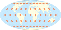
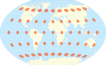
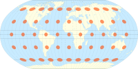
A single indicatrix describes the distortion at a single point. Because distortion varies across a map, generally Tissot's indicatrices are placed across a map to illustrate the spatial change in distortion. A common scheme places them at each intersection of displayed meridians and parallels. These schematics are important in the study of map projections, both to illustrate distortion and to provide the basis for the calculations that represent the magnitude of distortion precisely at each point.
There is a one-to-one correspondence between the Tissot indicatrix and the metric tensor of the map projection coordinate conversion.[1]
Description
Tissot's theory was developed in the context of cartographic analysis. Generally the geometric model represents the Earth, and comes in the form of a sphere or ellipsoid.
Tissot's indicatrices illustrate linear, angular, and areal distortions of maps:
- A map distorts distances (linear distortion) wherever the quotient between the lengths of an infinitesimally short line as projected onto the projection surface, and as it originally is on the Earth model, deviates from 1. The quotient is called the scale factor. Unless the projection is conformal at the point being considered, the scale factor varies by direction around the point.
- A map distorts angles wherever the angles measured on the model of the Earth are not conserved in the projection. This is expressed by an ellipse of distortion which is not a circle.
- A map distorts areas wherever areas measured in the model of the Earth are not conserved in the projection. This is expressed by ellipses of distortion whose areas vary across the map.
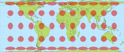
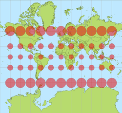
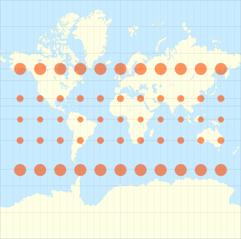
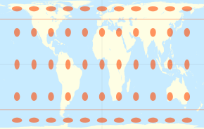
In conformal maps, where each point preserves angles projected from the geometric model, the Tissot's indicatrices are all circles of size varying by location, possibly also with varying orientation (given the four circle quadrants split by meridians and parallels). In equal-area projections, where area proportions between objects are conserved, the Tissot's indicatrices all have the same area, though their shapes and orientations vary with location. In arbitrary projections, both area and shape vary across the map.
| World maps comparing Tissot's indicatrices on some common projections |
|---|
|


Mathematics

In the adjacent image, ABCD is a circle with unit area defined in a spherical or ellipsoidal model of the Earth, and A′B′C′D′ is the Tissot's indicatrix that results from its projection onto the plane. Segment OA is transformed in OA′, and segment OB is transformed into OB′. Linear scale is not conserved along these two directions, since OA′ is not equal to OA and OB′ is not equal to OB. Angle MOA, in the unit area circle, is transformed in angle M′OA′ in the distortion ellipse. Because M′OA′ ≠ MOA, we know that there is an angular distortion. The area of circle ABCD is, by definition, equal to 1. Because the area of ellipse A′B′ is less than 1, a distortion of area has occurred.
In dealing with a Tissot indicatrix, different notions of radius come into play. The first is the infinitesimal radius of the original circle. The resulting ellipse of distortion will also have infinitesimal radius, but by the mathematics of differentials, the ratios of these infinitesimal values are finite. So, for example, if the resulting ellipse of distortion is the same size of infinitesimal as on the sphere, then its radius is considered to be 1. Lastly, the size that the indicatrix gets drawn for human inspection on the map is arbitrary. When an array of indicatrices is drawn on a map, they are all scaled by the same arbitrary amount so that their sizes are proportionally correct.
Like M in the diagram, the axes from O along the parallel and along the meridian may undergo a change of length and a rotation when projecting. It is common in the literature to represent scale along the meridian as h and scale along the parallel as k, for a given point. Likewise, the angle between meridian and parallel might have changed from 90° to some other value. Indeed, unless the map is conformal, all angles except the one subtended by the semi-major axis and semi-minor axis of the ellipse might have changed. A particular angle will have changed the most, and value of that maximum change is known as the angular deformation, denoted as θ′. Generally which angle that is and how it is oriented do not figure prominently in distortion analysis. It is the value of the change that is significant. The values of h, k, and θ′ can be computed as follows.[2]:24

where φ and λ are latitude and longitude, x and y are projected coordinates, and R is the radius of the globe.
As results, a and b represent the maximum and minimum scale factors at the point, which is the same thing as the semimajor and semiminor axes of the Tissot ellipse; s represents the amount of inflation or deflation in area (also given by a ∙ b); and ω represents the maximum angular distortion at the point.
For the Mercator projection, and any other conformal projection, h = k and θ′ = 90° so that each ellipse degenerates into a circle with the radius h = k being equal to the scale factor in any direction at that point.
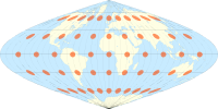
For the sinusoidal projection, and any other equal-area projection, the semi-major axis of the ellipse is the reciprocal of the semi-minor axis so that every ellipse has the same area even though their eccentricities vary.
For arbitrary projections, neither the shape nor the area of the ellipses are related to each other in general.[3]
An alternative derivation for numerical computation
Another way to understand and derive Tissot's indicatrix is through the differential geometry of surfaces.[4] This approach lends itself well to modern numerical methods, as the parameters of Tissot's indicatrix can be computed using singular value decomposition (SVD) and central difference approximation.
Differential distance on the ellipsoid
Let a 3D point, , on an ellipsoid be parameterized as:


where are longitude and latitude, respectively, and is a function of the equatorial radius, , and eccentricity, :


The element of distance on the sphere, is defined by the first fundamental form:


whose coefficients are defined as:

Computing the necessary derivatives gives:

where is a function of the equatorial radius, , and the ellipsoid eccentricity, :


Substituting these values into the first fundamental form gives the formula for elemental distance on the ellipsoid:

This result relates the measure of distance on the ellipsoid surface as a function of the spherical coordinate system.
Transforming the element of distance
Recall that the purpose of Tissot's indicatrix is to relate how distances on the sphere change when mapped to a planar surface. Specifically, the desired relation is the transform that relates differential distance along the bases of the spherical coordinate system to differential distance along the bases of the Cartesian coordinate system on the planar map. This can be expressed by the relation:


where and represent the computation of along the longitudinal and latitudinal axes, respectively. Computation of and can be performed directly from the equation above, yielding:


For the purposes of this computation, it is useful to express this relationship as a matrix operation:

Now, in order to relate the distances on the ellipsoid surface to those on the plane, we need to relate the coordinate systems. From the chain rule, we can write:

where J is the Jacobian matrix:

Plugging in the matrix expression for and yields the definition of the transform represented by the indicatrix:


This transform encapsulates the mapping from the ellipsoid surface to the plane. Expressed in this form, SVD can be used to parcel out the important components of the local transformation.
Numerical computation and SVD
In order to extract the desired distortion information, at any given location in the spherical coordinate system, the values of can be computed directly. The Jacobian, , can be computed analytically from the mapping function itself, but it is often simpler to numerically approximate the values at any location on the map using central differences. Once these values are computed, SVD can be applied to each transformation matrix to extract the local distortion information. Remember that, because distortion is local, every location on the map will have its own transformation.


Recall the definition of SVD:

It is the decomposition of the transformation, , into a rotation in the source domain (i.e. the ellipsoid surface), , a scaling along the basis, , and a subsequent second rotation, . For understanding distortion, the first rotation is irrelevant, as it rotates the axes of the circle but has no bearing on the final orientation of the ellipse. The next operation, represented by the diagonal singular value matrix, scales the circle along its axes, deforming it to an ellipse. Thus, the singular values represent the scale factors along axes of the ellipse. The first singular value provides the semi-major axis, , and the second provides the semi-minor axis, , which are the directional scaling factors of distortion. Scale distortion can be computed as the area of the ellipse, , or equivalently by the determinant of . Finally, the orientation of the ellipse, , can be extracted from the first column of as:


Gallery
 The transverse Mercator projection with Tissot's indicatrices
 The stereographic projection with Tissot's indicatrices
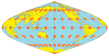 The sinusoidal projection with Tissot's indicatrices
 The Peirce quincuncial projection with Tissot's indicatrices
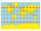 The Miller cylindrical projection with Tissot's indicatrices
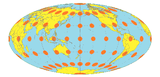 The Hammer projection with Tissot's indicatrices
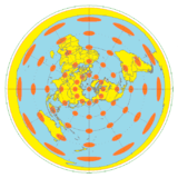 The azimuthal equidistant projection with Tissot's indicatrices
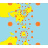
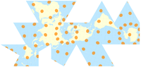 The Fuller projection with Tissot's indicatrices
See also
References
- Goldberg, David M.; Gott III, J. Richard (2007). "Flexion and Skewness in Map Projections of the Earth" (PDF). Cartographica. 42 (4): 297–318. arXiv:astro-ph/0608501. doi:10.3138/carto.42.4.297. Retrieved 2011-11-14.
- Snyder, John P. (1987). Map projections—A working manual. Professional Paper 1395. Denver: USGS. p. 383. ISBN 978-1782662228. Retrieved 2015-11-26.
- More general example of Tissot's indicatrix: the Winkel tripel projection.
- Laskowski, Piotr (1989). "The Traditional and Modern Look at Tissot's Indicatrix". The American Cartographer. 16 (2): 123–133.
External links
| Wikimedia Commons has media related to Map projections with Tissot's indicatrix. |