Smoothed-particle hydrodynamics
Smoothed-particle hydrodynamics (SPH) is a computational method used for simulating the mechanics of continuum media, such as solid mechanics and fluid flows. It was developed by Gingold and Monaghan [1] and Lucy[2] in 1977, initially for astrophysical problems. It has been used in many fields of research, including astrophysics, ballistics, volcanology, and oceanography. It is a meshfree Lagrangian method (where the co-ordinates move with the fluid), and the resolution of the method can easily be adjusted with respect to variables such as density.

Method
Advantages
- By construction, SPH is a meshfree method, which makes it ideally suited to simulate problems dominated by complex boundary dynamics, like free surface flows, or large boundary displacement.
- The lack of a mesh significantly simplifies the model implementation and its parallelization, even for many-core architectures.[3][4]
- SPH can be easily extended to a wide variety of fields, and hybridized with some other models, as discussed in Modelling Physics.
- As discussed in section on weakly compressible SPH, the method has great conservation features.
- The computational cost of SPH simulations per number of particles is significantly less than the cost of grid-based simulations per number of cells when the metric of interest is related to fluid density (e.g., the probability density function of density fluctuations).[5] This is the case because in SPH the resolution is put where the matter is.
Limitations
- Setting boundary conditions in SPH such as inlets and outlets [6] and walls [7] is more difficult than with grid-based methods. In fact, it has been stated that "the treatment of boundary conditions is certainly one of the most difficult technical points of the SPH method".[8] This challenge is partly because in SPH the particles near the boundary change with time.[9] Nonetheless, wall boundary conditions for SPH are available [7][9][10]
- The computational cost of SPH simulations per number of particles is significantly larger than the cost of grid-based simulations per number of cells when the metric of interest is not (directly) related to density (e.g., the kinetic-energy spectrum).[5] Therefore, overlooking issues of parallel speedup, the simulation of constant-density flows (e.g., external aerodynamics) is more efficient with grid-based methods than with SPH.
Examples
Fluid dynamics
Smoothed-particle hydrodynamics is being increasingly used to model fluid motion as well. This is due to several benefits over traditional grid-based techniques. First, SPH guarantees conservation of mass without extra computation since the particles themselves represent mass. Second, SPH computes pressure from weighted contributions of neighboring particles rather than by solving linear systems of equations. Finally, unlike grid-based techniques, which must track fluid boundaries, SPH creates a free surface for two-phase interacting fluids directly since the particles represent the denser fluid (usually water) and empty space represents the lighter fluid (usually air). For these reasons, it is possible to simulate fluid motion using SPH in real time. However, both grid-based and SPH techniques still require the generation of renderable free surface geometry using a polygonization technique such as metaballs and marching cubes, point splatting, or 'carpet' visualization. For gas dynamics it is more appropriate to use the kernel function itself to produce a rendering of gas column density (e.g., as done in the SPLASH visualisation package).
One drawback over grid-based techniques is the need for large numbers of particles to produce simulations of equivalent resolution. In the typical implementation of both uniform grids and SPH particle techniques, many voxels or particles will be used to fill water volumes that are never rendered. However, accuracy can be significantly higher with sophisticated grid-based techniques, especially those coupled with particle methods (such as particle level sets), since it is easier to enforce the incompressibility condition in these systems. SPH for fluid simulation is being used increasingly in real-time animation and games where accuracy is not as critical as interactivity.
Recent work in SPH for fluid simulation has increased performance, accuracy, and areas of application:
- B. Solenthaler, 2009, develops Predictive-Corrective SPH (PCISPH) to allow for better incompressibility constraints[11]
- M. Ihmsen et al., 2010, introduce boundary handling and adaptive time-stepping for PCISPH for accurate rigid body interactions[12]
- K. Bodin et al., 2011, replace the standard equation of state pressure with a density constraint and apply a variational time integrator[13]
- R. Hoetzlein, 2012, develops efficient GPU-based SPH for large scenes in Fluids v.3[14]
- N. Akinci et al., 2012, introduce a versatile boundary handling and two-way SPH-rigid coupling technique that is completely based on hydrodynamic forces; the approach is applicable to different types of SPH solvers [15]
- M. Macklin et al., 2013 simulates incompressible flows inside the Position Based Dynamics framework, for bigger timesteps [16]
- N. Akinci et al., 2013, introduce a versatile surface tension and two-way fluid-solid adhesion technique that allows simulating a variety of interesting physical effects that are observed in reality[17]
- J. Kyle and E. Terrell, 2013, apply SPH to Full-Film Lubrication[18]
- A. Mahdavi and N. Talebbeydokhti, 2015, propose a hybrid algorithm for implementation of solid boundary condition and simulate flow over a sharp crested weir[19]
- S. Tavakkol et al., 2016, develop curvSPH, which makes the horizontal and vertical size of particles independent and generates uniform mass distribution along curved boundaries[20]
- W. Kostorz and A. Esmail-Yakas, 2020, propose a general, efficient and simple method for piecewise-planar SPH wall boundary conditions[10] based on the semianalytical formulation of Kulasegaram et al.[21]
Astrophysics
Smoothed-particle hydrodynamics's adaptive resolution, numerical conservation of physically conserved quantities, and ability to simulate phenomena covering many orders of magnitude make it ideal for computations in theoretical astrophysics.[22]
Simulations of galaxy formation, star formation, stellar collisions,[23] supernovae[24] and meteor impacts are some of the wide variety of astrophysical and cosmological uses of this method.
SPH is used to model hydrodynamic flows, including possible effects of gravity. Incorporating other astrophysical processes which may be important, such as radiative transfer and magnetic fields is an active area of research in the astronomical community, and has had some limited success.[25][26]
Solid mechanics
Libersky and Petschek[27][28] extended SPH to Solid Mechanics. The main advantage of SPH in this application is the possibility of dealing with larger local distortion than grid-based methods. This feature has been exploited in many applications in Solid Mechanics: metal forming, impact, crack growth, fracture, fragmentation, etc.
Another important advantage of meshfree methods in general, and of SPH in particular, is that mesh dependence problems are naturally avoided given the meshfree nature of the method. In particular, mesh alignment is related to problems involving cracks and it is avoided in SPH due to the isotropic support of the kernel functions. However, classical SPH formulations suffer from tensile instabilities[29] and lack of consistency.[30] Over the past years, different corrections have been introduced to improve the accuracy of the SPH solution, leading to the RKPM by Liu et al.[31] Randles and Libersky[32] and Johnson and Beissel[33] tried to solve the consistency problem in their study of impact phenomena.
Dyka et al.[34][35] and Randles and Libersky[36] introduced the stress-point integration into SPH and Ted Belytschko et al.[37] showed that the stress-point technique removes the instability due to spurious singular modes, while tensile instabilities can be avoided by using a Lagrangian kernel. Many other recent studies can be found in the literature devoted to improve the convergence of the SPH method.
Recent improvements in understanding the convergence and stability of SPH have allowed for more widespread applications in Solid Mechanics. Other examples of applications and developments of the method include:
- Metal forming simulations.[38]
- SPH-based method SPAM (Smoothed Particle Applied Mechanics) for impact fracture in solids by William G. Hoover.[39]
- Modified SPH (SPH/MLSPH) for fracture and fragmentation.[40]
- Taylor-SPH (TSPH) for shock wave propagation in solids.[41]
- Generalized coordinate SPH (GSPH) allocates particles inhomogeneously in the Cartesian coordinate system and arranges them via mapping in a generalized coordinate system in which the particles are aligned at a uniform spacing.[42]
Numerical tools
Interpolations
The smoothed-particle hydrodynamics (SPH) method works by dividing the fluid into a set of discrete moving elements , referred to as particles. Their Lagrangian nature allows setting their position by integration of their velocity as:


These particles interact through a kernel function with characteristic radius known as the "smoothing length", typically represented in equations by . This means that the physical quantity of any particle can be obtained by summing the relevant properties of all the particles that lie within the range of the kernel, the latter being used as a weighting function . This can be understood in two steps. First an arbitrary field is written as a convolution with :


The error in making the above approximation is order . Secondly, the integral is approximated using a Riemann summation over the particles:


where the summation over includes all particles in the simulation. is the volume of particle , is the value of the quantity for particle and denotes position. For example, the density of particle can be expressed as:


where denotes the particle mass and the particle density, while is a short notation for . The error done in approximating the integral by a discrete sum depends on , on the particle size (i.e. , being the space dimension), and on the particle arrangement in space. The latter effect is still poorly known.[43]


Kernel functions commonly used include the Gaussian function, the quintic spline and the Wendland kernel.[44] The latter two kernels are compactly supported (unlike the Gaussian, where there is a small contribution at any finite distance away), with support proportional to . This has the advantage of saving computational effort by not including the relatively minor contributions from distant particles.

Although the size of the smoothing length can be fixed in both space and time, this does not take advantage of the full power of SPH. By assigning each particle its own smoothing length and allowing it to vary with time, the resolution of a simulation can be made to automatically adapt itself depending on local conditions. For example, in a very dense region where many particles are close together, the smoothing length can be made relatively short, yielding high spatial resolution. Conversely, in low-density regions where individual particles are far apart and the resolution is low, the smoothing length can be increased, optimising the computation for the regions of interest.
Operators
For particles of constant mass, differentiating the interpolated density with respect to time yields

where is the gradient of with respect to . Comparing the above equation with the continuity equation in continuum mechanics shows that the right-hand side is an approximation of ; hence one defines a discrete divergence operator as follows:


This operator gives an SPH approximation of at the particle for a given set of particles with given masses , positions and velocities .


Similarly, one can define a discrete gradient operator to approximate the pressure gradient at the position of particle :

where denote the set of particle pressures. There are several ways to define discrete operators in SPH; the above divergence and gradient formulae have the property to be skew-adjoint, leading to nice conservation properties.[45] On the other hand, while the divergence operator is zero-order consistent, it can be seen that the approximate gradient is not so. Several techniques have been proposed to circumvent this issue, leading to renormalised operators (see e.g.[46]).


Governing equations
The SPH operators can be used to discretize numbers of partial differential equations. For a compressible inviscid fluid, the Euler equations of mass conservation and momentum balance read:


All kinds of SPH divergence and gradient operators can practically be used for discretization purposes. Nevertheless, some perform better regarding physical and numerical effects. A frequently used form of the balance equations is based on the symmetric divergence operator and antisymmetric gradient:


Although there are several ways of discretizing the pressure gradient in the Euler equations, the above antisymmetric form is the most acknowledged one. It supports strict conservation of linear and angular momentum. This means that a force that is exerted on particle by particle equals the one that is exerted on particle by particle including the sign change of the effective direction, thanks to the antisymmetry property .
Variational principle
The above SPH governing equations can be derived from a Least action principle, starting from the Lagrangian of a particle system:
- ,

where is the particle specific internal energy. The Euler–Lagrange equation of variational mechanics reads, for each particle:


When applied to the above Lagrangian, it gives the following momentum equation:
- ,

where we used the thermodynamical property . Pluging the SPH density interpolation and differentiating explicitly leads to


which is the SPH momentum equation already mentioned, where we recognize the operator. This explains why linear momentum is conserved, and allows conservation of angular momentum and energy to be conserved as well.[47]
Time integration
From the work done in the 80's and 90's on numerical integration of point-like particles in large accelators, appropriate time integrators have been developed with accurate conservation properties on the long term; they are called symplectic integrators. The most popular in the SPH literature is the leapfrog scheme, which reads for each particle :

where is the time step, superscripts stand for time iterations while is the particle acceleration, given by the right-hand side of the momentum equation.


Other symplectic integrators exist (see the reference textbook [48]). It is recommended to use a symplectic (even low-order) scheme instead of a high order non-symplectic scheme, to avoid error accumulation after many iterations.
Integration of density has not been studied extensively (see below for more details).
Symplectic schemes are conservative but explicit, thus their numerical stability requires stability conditions, analogous to the Courant-Friedrichs-Lewy condition (see below).
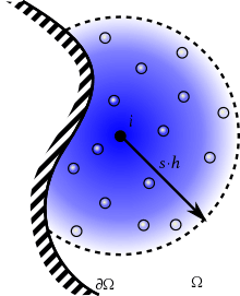
Boundary techniques

In case the SPH convolution shall be practised close to a boundary, i.e. closer than s · h, then the integral support is truncated. Indeed, when the convolution is affected by a boundary, the convolution shall be split in 2 integrals,

where B(r) is the compact support ball centered at r, with radius s · h, and Ω(r) denotes the part of the compact support inside the computational domain, Ω ∩ B(r). Hence, imposing boundary conditions in SPH is completely based on approximating the second integral on the right hand side. The same can be of course applied to the differential operators computation,

Several techniques has been introduced in the past to model boundaries in SPH.
Integral neglect
The most straightforward boundary model is neglecting the integral,

such that just the bulk interactions are taken into account,

This is a popular approach when free-surface is considered in monophase simulations.[49]
The main benefit of this boundary condition is its obvious simplicity. However, several consistency issues shall be considered when this boundary technique is applied.[49] That's in fact a heavy limitation on its potential applications.
Fluid Extension
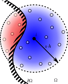
Probably the most popular methodology, or at least the most traditional one, to impose boundary conditions in SPH, is Fluid Extension technique. Such technique is based on populating the compact support across the boundary with so-called ghost particles, conveniently imposing their field values.[50]
Along this line, the integral neglect methodology can be considered as a particular case of fluid extensions, where the field, A, vanish outside the computational domain.
The main benefit of this methodology is the simplicity, provided that the boundary contribution is computed as part of the bulk interactions. Also, this methodology has been deeply analysed in the literature.[51][50][52]
On the other hand, deploying ghost particles in the truncated domain is not a trivial task, such that modelling complex boundary shapes becomes cumbersome. The 2 most popular approaches to populate the empty domain with ghost particles are Mirrored-Particles [53] and Fixed-Particles.[50]
Boundary Integral
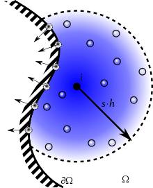
The newest Boundary technique is the Boundary Integral methodology.[54] In this methodology, the empty volume integral is replaced by a surface integral, and a renormalization:


with nj the normal of the generic jth boundary element. The surface term can be also solved considering a semi-analytic expression.[54]
Modelling Physics
Hydrodynamics
Weakly compressible approach
Another way to determine the density is based on the SPH smoothing operator itself. Therefore, the density is estimated from the particle distribution utilizing the SPH interpolation. To overcome undesired errors at the free surface through kernel truncation, the density formulation can again be integrated in time. [54]
The weakly compressible SPH in fluid dynamics is based on the discretization of the Navier–Stokes equations or Euler equations for compressible fluids. To close the system, an appropriate equation of state is utilized to link pressure and density . Generally, the so-called Cole equation [55] (sometimes mistakenly referred to as the "Tait equation") is used in SPH. It reads


where is the reference density and the speed of sound. For water, is commonly used. The background pressure is added to avoid negative pressure values.


Real nearly incompressible fluids such as water are characterised by very high speed of sounds of the order . Hence, pressure information travels fast compared to the actual bulk flow, which leads to very small Mach numbers . The momentum equation leads to the following relation:


where is the density change and the velocity vector. In practice a value of c smaller than the real one is adopted to avoid time steps too small in the time integration scheme. Generally a numerical speed of sound is adopted such that density variation smaller than 1% are allowed. This is the so-called weak-compressibility assumption. This corresponds to a Mach number smaller than 0.1, which implies:


where the maximum velocity needs to be estimated, for e.g. by Torricelli's law or an educated guess. Since only small density variations occur, a linear equation of state can be adopted:[56]


Usually the weakly-compressible schemes are affected by a high-frequency spurious noise on the pressure and density fields. [57] This phenomenon is caused by the nonlinear interaction of acoustic waves and by fact that the scheme is explicit in time and centred in space .[58]
Through the years, several techniques have been proposed to get rid of this problem. They can be classified in three different groups:
- the schemes that adopt density filters,
- the models that add a diffusive term in the continuity equation,
- the schemes that employ Riemann Solvers to model the particle interaction.
The schemes of the first group apply a filter directly on the density field to remove the spurious numerical noise. The most used filters are the MLS (Moving Least Squares) and the Shepard filter [57] which can be applied at each time step or every n time steps. The more frequent is the use of the filtering procedure, the more regular density and pressure fields are obtained. On the other hand, this leads to an increase of the computational costs. In long time simulations, the use of the filtering procedure may lead to the disruption of the hydrostatic pressure component and to an inconsistency between the global volume of fluid and the density field. Further, it does not ensure the enforcement of the dynamic free-surface boundary condition.
A different way to smooth out the density and pressure field is to add a diffusive term inside the continuity equation (group 2) :

The first schemes that adopted such an approach were described in Ferrari [59] and in Molteni[56] where the diffusive term was modelled as a Laplacian of the density field. A similar approach was also used in [60] .
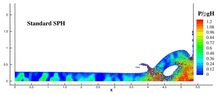
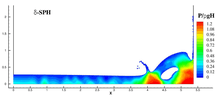
In [61] a correction to the diffusive term of Molteni[56] was proposed to remove some inconsistencies close to the free-surface. In this case the adopted diffusive term is equivalent to a high-order differential operator on the density field .[62] The scheme is called δ-SPH and preserves all the conservations properties of the SPH without diffusion (e.g., linear and angular momenta, total energy, see [63] ) along with a smooth and regular representation of the density and pressure fields.
In the third group there are those SPH schemes which employ numerical fluxes obtained through Riemann solvers to model the particle interactions [64] [65] .[66]
Incompressible approach
Viscosity modelling
In general, the description of hydrodynamic flows require a convenient treatment of diffusive processes to model the viscosity in the Navier–Stokes equations. It needs special consideration because it involves the laplacian differential operator. Since the direct computation does not provide satisfactory results, several approaches to model the diffusion have been proposed.
- Artificial viscosity
Introduced by Monaghan and Gingold [67] the artificial viscosity was used to deal with high Mach number fluid flows. It reads

Here, is controlling a volume viscosity while acts similar to the Neumann Richtmeyr artificial viscosity. The is defined by


The artificial viscosity also has shown to improve the overall stability of general flow simulations. Therefore, it is applied to inviscid problems in the following form

It is possible to not only stabilize inviscid simulations but also to model the physical viscosity by this approach. To do so

is substituted in the equation above, where is the number of spartial dimensions of the model. This approach introduces the bulk viscosity .


- Morris
For low Reynolds numbers the viscosity model by Morris [68] was proposed.

- LoShao
Additional physics
- Surface Tension
- Heat transfer
- Turbulence
Multiphase extensions
Astrophysics
Often in astrophysics, one wishes to model self-gravity in addition to pure hydrodynamics. The particle-based nature of SPH makes it ideal to combine with a particle-based gravity solver, for instance tree gravity code,[69] particle mesh, or particle-particle particle-mesh.
Solid mechanics
Others
The discrete element method, used for simulating granular materials, is related to SPH.
Variants of the method
References
- R.A. Gingold; J.J. Monaghan (1977). "Smoothed particle hydrodynamics: theory and application to non-spherical stars". Mon. Not. R. Astron. Soc. 181 (3): 375–89. Bibcode:1977MNRAS.181..375G. doi:10.1093/mnras/181.3.375.
- L.B. Lucy (1977). "A numerical approach to the testing of the fission hypothesis". Astron. J. 82: 1013–1024. Bibcode:1977AJ.....82.1013L. doi:10.1086/112164.
- Takahiro Harada; Seiichi Koshizuka; Yoichiro Kawaguchi (2007). Smoothed particle hydrodynamics on GPUs. Computer Graphics International. pp. 63–70.
- Alejandro Crespo; Jose M. Dominguez; Anxo Barreiro; Moncho Gomez-Gesteira; Benedict D. Rogers (2011). "GPUs, a new tool of acceleration in CFD: efficiency and reliability on smoothed particle hydrodynamics methods". PLOS One. 6 (6): e20685. Bibcode:2011PLoSO...620685C. doi:10.1371/journal.pone.0020685. PMC 3113801. PMID 21695185.
- Price, D. J. (2011). "Smoothed Particle Hydrodynamics: Things I wish my mother taught me". Advances in Computational Astrophysics: Methods. 453: 249. arXiv:1111.1259. Bibcode:2012ASPC..453..249P.
- "The Smoothed Particle Hydrodynamics Method vs. Finite Volume Numerical Methods". 2018-03-21. Retrieved 2018-08-30.
- Adami, S. and Hu, X. Y. and Adams, N. A.. (2012). "A generalized wall boundary condition for smoothed particle hydrodynamics". Journal of Computational Physics. 231 (21): 7057–7075. Bibcode:2012JCoPh.231.7057A. doi:10.1016/j.jcp.2012.05.005.CS1 maint: multiple names: authors list (link)
- Shadloo, M. S. and Oger, G. and Touze, D. L.. (2016). "Smoothed particle hydrodynamics method for fluid flows, towards industrial applications: Motivations, current state, and challenges". Computers and Fluids. 136: 11–34. doi:10.1016/j.compfluid.2016.05.029.CS1 maint: multiple names: authors list (link)
- Fraser, K.and Kiss, L. I. and St-George, L. (2016). "A generalized wall boundary condition for smoothed particle hydrodynamics". 14th International LS-DYNA Conference.CS1 maint: multiple names: authors list (link)
- Kostorz (2020). "A semi-analytical boundary integral method for radial functions with application to Smoothed Particle Hydrodynamics". Journal of Computational Physics. 417. doi:10.1016/j.jcp.2020.109565.
-
Solenthaler (2009). "Predictive-Corrective Incompressible SPH". Cite journal requires
|journal=(help) - Imhsen (2010). "Boundary handling and adaptive time-stepping for PCISPH". Workshop on Virtual Reality Interaction and Physical Simulation VRIPHYS.
- Bodin (2011). "Constraint Fluids". IEEE Transactions on Visualization and Computer Graphics. 18 (3): 516–26. doi:10.1109/TVCG.2011.29. PMID 22241284.
- Hoetzlein (2012). "Fluids v.3, A Large scale, Open Source Fluid Simulator". Cite journal requires
|journal=(help) - Akinci (2012). "Versatile Rigid-Fluid Coupling for Incompressible SPH". ACM Transactions on Graphics. 31 (4): 1–8. doi:10.1145/2185520.2185558.
- Macklin (2013). "Position Based Fluids". ACM Transactions on Graphics. 32 (4): 1. doi:10.1145/2461912.2461984.
- Akinci (2013). "Versatile Surface Tension and Adhesion for SPH Fluids SPH". ACM Transactions on Graphics. 32 (6): 1–8. CiteSeerX 10.1.1.462.8293. doi:10.1145/2508363.2508395.
- Journal of Tribology (2013). "Application of Smoothed Particle Hydrodynamics to Full-Film Lubrication". Cite journal requires
|journal=(help) - Mahdavi and Talebbeydokhti (2015). "A hybrid solid boundary treatment algorithm for smoothed particle hydrodynamics". Scientia Iranica, Transaction A, Civil Engineering. 22 (4): 1457–1469.
- International Journal for Numerical Methods in Fluids (2016). "Curvilinear smoothed particle hydrodynamics". International Journal for Numerical Methods in Fluids. 83 (2): 115–131. Bibcode:2017IJNMF..83..115T. doi:10.1002/fld.4261.
- Kulasegaram (2004). "A variational formulation based contact algorithm for rigid boundaries in two-dimensional SPH applications". Computational Mechanics. 33 (4): 316–325. doi:10.1007/s00466-003-0534-0.
- Price, Daniel J (2009). "Astrophysical Smooth Particle Hydrodynamics". New Astron.rev. 53 (4–6): 78–104. arXiv:0903.5075. Bibcode:2009NewAR..53...78R. doi:10.1016/j.newar.2009.08.007.
- Rosswog, Stephan (2015). "SPH Methods in the Modelling of Compact Objects". Living Rev Comput Astrophys. 1 (1): 1. arXiv:1406.4224. Bibcode:2015LRCA....1....1R. doi:10.1007/lrca-2015-1.
- Price, Daniel J; Rockefeller, Gabriel; Warren, Michael S (2006). "SNSPH: A Parallel 3-D Smoothed Particle Radiation Hydrodynamics Code". Astrophys. J. 643: 292–305. arXiv:astro-ph/0512532. doi:10.1086/501493.
- "Star Formation with Radiative Transfer".
- http://users.monash.edu.au/~dprice/pubs/spmhd/price-spmhd.pdf
- Libersky, L.D.; Petschek, A.G. (1990). Smooth Particle Hydrodynamics with Strength of Materials, Advances in the Free Lagrange Method. Lecture Notes in Physics. 395. pp. 248–257. doi:10.1007/3-540-54960-9_58. ISBN 978-3-540-54960-4.
- L.D. Libersky; A.G. Petschek; A.G. Carney; T.C. Hipp; J.R. Allahdadi; F.A. High (1993). "Strain Lagrangian hydrodynamics: a three-dimensional SPH code for dynamic material response". J. Comput. Phys. 109 (1): 67–75. Bibcode:1993JCoPh.109...67L. doi:10.1006/jcph.1993.1199.
- J.W. Swegle; D.A. Hicks; S.W. Attaway (1995). "Smooth particle hydrodynamics stability analysis". J. Comput. Phys. 116 (1): 123–134. Bibcode:1995JCoPh.116..123S. doi:10.1006/jcph.1995.1010.
- T. Belytschko; Y. Krongauz; J. Dolbow; C. Gerlach (1998). "On the completeness of meshfree particle methods". Int. J. Numer. Methods Eng. 43 (5): 785–819. Bibcode:1998IJNME..43..785B. CiteSeerX 10.1.1.28.491. doi:10.1002/(sici)1097-0207(19981115)43:5<785::aid-nme420>3.0.co;2-9.
- W.K. Liu; S. Jun; Y.F. Zhang (1995). "Reproducing kernel particle methods". Int. J. Numer. Methods Eng. 20 (8–9): 1081–1106. Bibcode:1995IJNMF..20.1081L. doi:10.1002/fld.1650200824.
- P.W. Randles; L.D. Libersky (1997). "Recent improvements in SPH modelling of hypervelocity impact". Int. J. Impact Eng. 20 (6–10): 525–532. doi:10.1016/s0734-743x(97)87441-6.
- G.R. Johnson; S.R. Beissel (1996). "Normalized smoothing functions for SPH impact computations". Int. J. Numer. Methods Eng. 39 (16): 2725–2741. Bibcode:1996IJNME..39.2725J. doi:10.1002/(sici)1097-0207(19960830)39:16<2725::aid-nme973>3.0.co;2-9.
- C.T. Dyka; R.P. Ingel (1995). "An approach for tension instability in Smoothed Particle Hydrodynamics". Comput. Struct. 57 (4): 573–580. doi:10.1016/0045-7949(95)00059-p.
- C.T. Dyka; P.W. Randles; R.P. Ingel (1997). "Stress points for tension instability in SPH". Int. J. Numer. Methods Eng. 40 (13): 2325–2341. Bibcode:1997IJNME..40.2325D. doi:10.1002/(sici)1097-0207(19970715)40:13<2325::aid-nme161>3.0.co;2-8.
- P.W. Randles; L.D. Libersky (2000). "Normalized SPH with stress points". Int. J. Numer. Methods Eng. 48 (10): 1445–1462. Bibcode:2000IJNME..48.1445R. doi:10.1002/1097-0207(20000810)48:10<1445::aid-nme831>3.0.co;2-9.
- T. Belytschko; Y. Guo; W.K. Liu; S.P. Xiao (2000). "A unified stability analysis of meshless particle methods". Int. J. Numer. Methods Eng. 48 (9): 1359–1400. Bibcode:2000IJNME..48.1359B. doi:10.1002/1097-0207(20000730)48:9<1359::aid-nme829>3.0.co;2-u.
- J. Bonet; S. Kulasegaram (2000). "Correction and stabilization of smooth particle hydrodynamics methods with applications in metal forming simulations". Int. J. Numer. Methods Eng. 47 (6): 1189–1214. Bibcode:2000IJNME..47.1189B. doi:10.1002/(sici)1097-0207(20000228)47:6<1189::aid-nme830>3.0.co;2-i.
- W. G. Hoover; C. G. Hoover (2001). "SPAM-based recipes for continuum simulations". Computing in Science and Engineering. 3 (2): 78–85. Bibcode:2001CSE.....3b..78H. doi:10.1109/5992.909007.
- T. Rabczuk; J. Eibl; L. Stempniewski (2003). "Simulation of high velocity concrete fragmentation using SPH/MLSPH". Int. J. Numer. Methods Eng. 56 (10): 1421–1444. Bibcode:2003IJNME..56.1421R. doi:10.1002/nme.617.
- M.I. Herreros; M. Mabssout (2011). "A two-steps time discretization scheme using the SPH method for shock wave propagation". Comput. Methods Appl. Mech. Engrg. 200 (21–22): 1833–1845. Bibcode:2011CMAME.200.1833H. doi:10.1016/j.cma.2011.02.006.
- S. Yashiro; T. Okabe (2015). "Smoothed particle hydrodynamics in a generalized coordinate system with a finite-deformation constitutive model". Int. J. Numer. Methods Eng. 103 (11): 781–797. Bibcode:2015IJNME.103..781Y. doi:10.1002/nme.4906.
- N.J. Quinlan; M. Basa; M. Lastiwka (2006). "Truncation error in mesh-free particle methods" (PDF). International Journal for Numerical Methods in Engineering. 66 (13): 2064–2085. Bibcode:2006IJNME..66.2064Q. doi:10.1002/nme.1617. hdl:10379/1170.
- H. Wendland (1995). "Piecewise polynomial, positive definite and compactly supported radial functions of minimal degree". Advances in Computational Mathematics. 4 (4): 389–396. doi:10.1007/BF02123482.
- A. Mayrhofer; B.D. Rogers; D. Violeau; M. Ferrand (2013). "Investigation of wall bounded flows using SPH and the unified semi-analytical wall boundary conditions". Computer Physics Communications. 184 (11): 2515–2527. arXiv:1304.3692. Bibcode:2013CoPhC.184.2515M. CiteSeerX 10.1.1.770.4985. doi:10.1016/j.cpc.2013.07.004.
- J. Bonet; T.S. Lok (1999). "Variational and momentum preservation aspects of Smoothed Particle Hydrodynamics formulations". Computers Methods in Applied Mechanical Engineering. 180 (1–2): 97–115. Bibcode:1999CMAME.180...97B. doi:10.1016/S0045-7825(99)00051-1.
- J.J. Monaghan (2005). "Smoothed particle hydrodynamics". Reports on Progress in Physics. 68 (8): 1703–1759. Bibcode:2005RPPh...68.1703M. doi:10.1088/0034-4885/68/8/R01.
- E. Hairer; C. Lubich; G. Wanner (2006). Geometric Numerical Integration. Springer. ISBN 978-3-540-30666-5.
- Andrea Colagrossi; Matteo Antuono; David Le Touzè (2009). "Theoretical considerations on the free-surface role in the smoothed-particle-hydrodynamics model". Physical Review E. 79 (5): 056701. Bibcode:2009PhRvE..79e6701C. doi:10.1103/PhysRevE.79.056701. PMID 19518587.
- Bejamin Bouscasse; Andrea Colagrossi; Salvatore Marrone; Matteo Antuono (2013). "Nonlinear water wave interaction with floating bodies in SPH". Journal of Fluids and Structures. 42: 112–129. Bibcode:2013JFS....42..112B. doi:10.1016/j.jfluidstructs.2013.05.010.
- Fabricio Macià; Matteo Antuono; Leo M González; Andrea Colagrossi (2011). "Theoretical analysis of the no-slip boundary condition enforcement in SPH methods". Progress of Theoretical Physics. 125 (6): 1091–1121. Bibcode:2011PThPh.125.1091M. doi:10.1143/PTP.125.1091.
- Jose Luis Cercos-Pita; Matteo Antuono; Andrea Colagrossi; Antonio Souto (2017). "SPH energy conservation for fluid--solid interactions". Computer Methods in Applied Mechanics and Engineering. 317: 771–791. Bibcode:2017CMAME.317..771C. doi:10.1016/j.cma.2016.12.037.
- J. Campbell; R. Vignjevic; L. Libersky (2000). "A contact algorithm for smoothed particle hydrodynamics". Computer Methods in Applied Mechanics and Engineering. 184 (1): 49–65. Bibcode:2000CMAME.184...49C. doi:10.1016/S0045-7825(99)00442-9.
- M. Ferrand, D.R. Laurence, B.D. Rogers, D. Violeau, C. Kassiotis (2013). "Unified semi-analytical wall boundary conditions for inviscid, laminar or turbulent flows in the meshless SPH method". International Journal for Numerical Methods in Fluids. Int. J. Numer. Meth. Fluids. 71 (4): 446–472. Bibcode:2013IJNMF..71..446F. doi:10.1002/fld.3666.CS1 maint: multiple names: authors list (link)
- H. R. Cole (1948). Underwater Explosions. Princeton, New Jersey: Princeton University Press.
- D. Molteni, A. Colagrossi (2009). "A simple procedure to improve the pressure evaluation in hydrodynamic context using the SPH". Computer Physics Communications. 180 (6): 861–872. Bibcode:2009CoPhC.180..861M. doi:10.1016/j.cpc.2008.12.004.
- Colagrossi, Andrea; Landrini, Maurizio (2003). "Numerical simulation of interfacial flows by smoothed particle hydrodynamics". Journal of Computational Physics. 191 (2): 448–475. Bibcode:2003JCoPh.191..448C. doi:10.1016/S0021-9991(03)00324-3.
- Randall J. LeVeque (2007). Finite difference methods for ordinary and partial differential equations: steady-state and time-dependent problems. Siam.
- A. Ferrari, M. Dumbser, E. Toro, A. Armanini (2009). "A new 3D parallel SPH scheme for free surface flows". Computers & Fluids. Elsevier. 38 (6): 1203–1217. doi:10.1016/j.compfluid.2008.11.012.CS1 maint: multiple names: authors list (link)
- Fatehi, R and Manzari, MT (2011). "A remedy for numerical oscillations in weakly compressible smoothed particle hydrodynamics". International Journal for Numerical Methods in Fluids. Wiley Online Library. 67 (9): 1100–1114. Bibcode:2011IJNMF..67.1100F. doi:10.1002/fld.2406.CS1 maint: multiple names: authors list (link)
- M. Antuono, A. Colagrossi, S. Marrone, D. Molteni (2010). "Free-surface flows solved by means of SPH schemes with numerical diffusive terms". Computer Physics Communications. Elsevier. 181 (3): 532–549. Bibcode:2010CoPhC.181..532A. doi:10.1016/j.cpc.2009.11.002.CS1 maint: multiple names: authors list (link)
- M. Antuono, A. Colagrossi, S. Marrone (2012). "Numerical diffusive terms in weakly-compressible SPH schemes". Computer Physics Communications. Elsevier. 183 (12): 2570–2580. Bibcode:2012CoPhC.183.2570A. doi:10.1016/j.cpc.2012.07.006.CS1 maint: multiple names: authors list (link)
- Antuono Matteo and Marrone S and Colagrossi A and Bouscasse B (2015). "Energy balance in the $\delta$-SPH scheme". Computer Methods in Applied Mechanics and Engineering. Elsevier. 289: 209–226. doi:10.1016/j.cma.2015.02.004.
- JP. Vila (1999). "On particle weighted methods and smooth particle hydrodynamics". Mathematical Models and Methods in Applied Sciences. World Scientific. 9 (2): 161–209. doi:10.1142/S0218202599000117.
- Marongiu Jean-Christophe and Leboeuf Francis and Caro Joëlle and Parkinson Etienne (2010). "Free surface flows simulations in Pelton turbines using an hybrid SPH-ALE method" (PDF). Journal of Hydraulic Research. Taylor & Francis. 48 (S1): 40–49. doi:10.1080/00221686.2010.9641244.
- De Leffe, Matthieu (2011). Modelisation d'écoulements visqueux par methode SPH en vue d'application à l'hydrodynamique navale. PhD Thesis, Ecole centrale de Nantes.
- J.J. Monaghan; R.A. Gingold (1983). "Shock Simulation by the Particle Method". Journal of Computational Physics. 52 (2): 347–389. Bibcode:1983JCoPh..52..374M. doi:10.1016/0021-9991(83)90036-0.
- J.P. Morris; P.J. Fox; Y. Zhu (1997). "Modeling Low Reynolds Number Incompressible Flows Using SPH". Journal of Computational Physics. 136 (1): 214–226. Bibcode:1997JCoPh.136..214M. doi:10.1006/jcph.1997.5776.
- Marios D. Dikaiakos; Joachim Stadel, PKDGRAV The Parallel k-D Tree Gravity Code, retrieved February 1, 2017
Further reading
- Hoover, W. G. (2006). Smooth Particle Applied Mechanics: The State of the Art, World Scientific.
- Impact Modelling with SPH Stellingwerf, R. F., Wingate, C. A., Memorie della Societa Astronomia Italiana, Vol. 65, p. 1117 (1994).
- Amada, T., Imura, M., Yasumuro, Y., Manabe, Y. and Chihara, K. (2004) Particle-based fluid simulation on GPU, in proceedings of ACM Workshop on General-purpose Computing on Graphics Processors (August, 2004, Los Angeles, California).
- Desbrun, M. and Cani, M-P. (1996). Smoothed Particles: a new paradigm for animating highly deformable bodies. In Proceedings of Eurographics Workshop on Computer Animation and Simulation (August 1996, Poitiers, France).
- Hegeman, K., Carr, N.A. and Miller, G.S.P. Particle-based fluid simulation on the GPU. In Proceedings of International Conference on Computational Science (Reading, UK, May 2006). Proceedings published as Lecture Notes in Computer Science v. 3994/2006 (Springer-Verlag).
- M. Kelager. (2006) Lagrangian Fluid Dynamics Using Smoothed Particle Hydrodynamics, M. Kelagar (MS Thesis, Univ. Copenhagen).
- Kolb, A. and Cuntz, N. (2005). Dynamic particle coupling for GPU-based fluid simulation. In Proceedings of the 18th Symposium on Simulation Techniques (2005) pp. 722–727.
- Liu, G.R. and Liu, M.B. Smoothed Particle Hydrodynamics: a meshfree particle method. Singapore: World Scientific (2003).
- Monaghan, J.J. (1992). Smoothed Particle Hydrodynamics. Annu. Rev. Astron. Astrophys. (1992). 30 : 543–74.
- Muller, M., Charypar, D. and Gross, M. Particle-based Fluid Simulation for Interactive Applications, In Proceedings of Eurographics/SIGGRAPH Symposium on Computer Animation (2003), eds. D. Breen and M. Lin.
- Vesterlund, M. Simulation and Rendering of a Viscous Fluid Using Smoothed Particle Hydrodynamics, (MS Thesis, Umea University, Sweden).
- Violeau, D., Fluid Mechanics and the SPH method. Oxford University Press (2012).
External links
- First large simulation of star formation using SPH
- SPHERIC (SPH rEsearch and engineeRing International Community)
- ITVO is the web-site of The Italian Theoretical Virtual Observatory created to query a database of numerical simulation archive.
- SPHC Image Gallery depicts a wide variety of test cases, experimental validations, and commercial applications of the SPH code SPHC.
- A derivation of the SPH model starting from Navier-Stokes equations
Software
- Algodoo is a 2D simulation framework for education using SPH
- AQUAgpusph is the free (GPLv3) SPH of the researchers, by the researchers, for the researchers
- dive solutions is a commercial web-based SPH engineering software for CFD purposes
- DualSPHysics is a mostly open source SPH code based on SPHysics and using GPU computing. The open source components are available under the LGPL.
- FLUIDS v.1 is a simple, open source (Zlib), real-time 3D SPH implementation in C++ for liquids for CPU and GPU.
- Fluidix is a GPU-based particle simulation API available from OneZero Software
- GADGET is a freely available (GPL) code for cosmological N-body/SPH simulations
- GPUSPH SPH simulator with viscosity (GPLv3)
- Pasimodo is a program package for particle-based simulation methods, e.g. SPH
- Physics Abstraction Layer is an open source abstraction system that supports real time physics engines with SPH support
- PreonLab is a commercial engineering software developed by FIFTY2 Technology implementing an implicit SPH method
- Punto is a freely available visualisation tool for particle simulations
- pysph Open Source Framework for Smoothed Particle Hydrodynamics in Python (New BSD License)
- SimPARTIX is a commercial simulation package for SPH and DEM simulations from Fraunhofer IWM
- SPH-flow
- SPHERA
- SPHysics is an open source SPH implementation in Fortran
- SPLASH is an open source (GPL) visualisation tool for SPH simulations
- SYMPLER: A freeware SYMbolic ParticLE simulatoR from the University of Freiburg.
- Nauticle is a general-purpose computational tool for particle-based numerical methods.