Small-angle approximation
The small-angle approximation is a useful simplification of the basic trigonometric functions which is approximately true in the limit where the angle approaches zero. They are truncations of the Taylor series for the basic trigonometric functions to a second-order approximation. This truncation gives:[1][2]


where θ is the angle in radians.
The small angle approximation is useful in many areas of engineering and physics, including mechanics, electromagnetics, optics (where it forms the basis of the paraxial approximation), cartography, astronomy, computer science, and so on.
Justifications
Graphic
The accuracy of the approximations can be seen below in Figure 1 and Figure 2. As the angle approaches zero, it is clear that the gap between the approximation and the original function quickly vanishes.
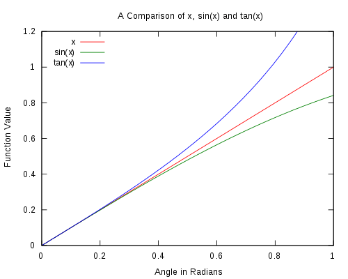 Figure 1. A comparison of the basic odd trigonometric functions to θ. It is seen that as the angle approaches 0 the approximations become better.
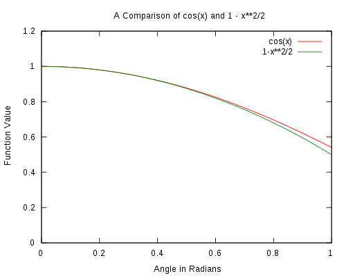 Figure 2. A comparison of cos θ to 1 − θ2/2. It is seen that as the angle approaches 0 the approximation becomes better.
Geometric

The red section on the right, d, is the difference between the lengths of the hypotenuse, H, and the adjacent side, A. As is shown, H and A are almost the same length, meaning cos θ is close to 1 and θ2/2 helps trim the red away.

The opposite leg, O, is approximately equal to the length of the blue arc, s. Gathering facts from geometry, s = Aθ, from trigonometry, sin θ = O/H and tan θ = O/A, and from the picture, O ≈ s and H ≈ A leads to:

Simplifying leaves,

Calculus
Using the squeeze theorem,[3] we can prove that which is a formal restatement of the approximation for small values of θ.


A more careful application of the squeeze theorem proves that from which we conclude that for small values of θ.


Finally, using L'Hôpital's rule tells us that which rearranges algebraically to give for small values of θ.


Algebraic
The Maclaurin expansion (the Taylor expansion about 0) of the relevant trigonometric function is[4]

where θ is the angle in radians. In clearer terms,

It is readily seen that the second most significant (third-order) term falls off as the cube of the first term; thus, even for a not-so-small argument such as 0.01, the value of the second most significant term is on the order of 0.000001, or 1/10000 the first term. One can thus safely approximate:

By extension, since the cosine of a small angle is very nearly 1, and the tangent is given by the sine divided by the cosine,
- ,

Error of the approximations
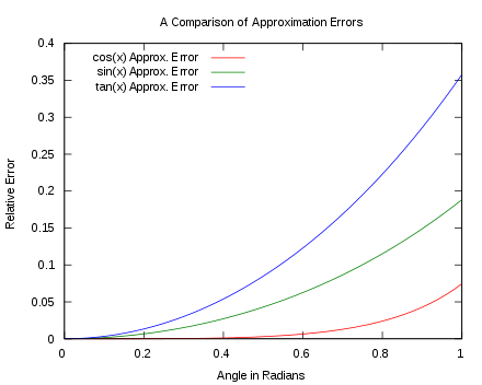
Figure 3 shows the relative errors of the small angle approximations. The angles at which the relative error exceeds 1% are as follows:
- tan θ ≈ θ at about 0.176 radians (10°).
- sin θ ≈ θ at about 0.244 radians (14°).
- cos θ ≈ 1 − θ2/2 at about 0.664 radians (38°).
Angle sum and difference
The angle addition and subtraction theorems reduce to the following when one of the angles is small (β ≈ 0):
cos(α + β) ≈ cos(α) - βsin(α), cos(α - β) ≈ cos(α) + βsin(α), sin(α + β) ≈ sin(α) + βcos(α), sin(α - β) ≈ sin(α) - βcos(α).
Specific uses
Astronomy
In astronomy, the angular size or angle subtended by the image of a distant object is often only a few arcseconds, so it is well suited to the small angle approximation.[5] The linear size (D) is related to the angular size (X) and the distance from the observer (d) by the simple formula:

where X is measured in arcseconds.
The number 206265 is approximately equal to the number of arcseconds in a circle (1296000), divided by 2π.
The exact formula is

and the above approximation follows when tan X is replaced by X.
Motion of a pendulum
The second-order cosine approximation is especially useful in calculating the potential energy of a pendulum, which can then be applied with a Lagrangian to find the indirect (energy) equation of motion.
When calculating the period of a simple pendulum, the small-angle approximation for sine is used to allow the resulting differential equation to be solved easily by comparison with the differential equation describing simple harmonic motion.
Structural mechanics
The small-angle approximation also appears in structural mechanics, especially in stability and bifurcation analyses (mainly of axially-loaded columns ready to undergo buckling). This leads to significant simplifications, though at a cost in accuracy and insight into the true behavior.
Piloting
The 1 in 60 rule used in air navigation has its basis in the small-angle approximation, plus the fact that one radian is approximately 60 degrees.
Interpolation
The formulas for addition and subtraction involving a small angle may be used for interpolating between trigonometric table values:
Example: sin(0.755)
sin(0.755) = sin(0.75 + 0.005) ≈ sin(0.75) + (0.005)cos(0.75) ≈ (0.6816) + (0.005)(0.7317) [Obtained sin(0.75) and cos(0.75) values from trigonometric table] ≈ 0.6853.
See also
- Skinny triangle
- Infinitesimal oscillations of a pendulum
- Versine and haversine
- Exsecant and excosecant
References
- Holbrow, Charles H.; et al. (2010), Modern Introductory Physics (2nd ed.), Springer Science & Business Media, pp. 30–32, ISBN 0387790799.
- Plesha, Michael; et al. (2012), Engineering Mechanics: Statics and Dynamics (2nd ed.), McGraw-Hill Higher Education, p. 12, ISBN 0077570618.
- Larson, Ron; et al. (2006), Calculus of a Single Variable: Early Transcendental Functions (4th ed.), Cengage Learning, p. 85, ISBN 0618606254.
- Boas, Mary L. (2006). Mathematical Methods in the Physical Sciences. Wiley. p. 26. ISBN 978-0-471-19826-0.
- Green, Robin M. (1985), Spherical Astronomy, Cambridge University Press, p. 19, ISBN 0521317797.