Pendulum (mathematics)
A pendulum is a body suspended from a fixed support so that it swings freely back and forth under the influence of gravity. When a pendulum is displaced sideways from its resting, equilibrium position, it is subject to a restoring force due to gravity that will accelerate it back toward the equilibrium position. When released, the restoring force acting on the pendulum's mass causes it to oscillate about the equilibrium position, swinging it back and forth. The mathematics of pendulums are in general quite complicated. Simplifying assumptions can be made, which in the case of a simple pendulum allow the equations of motion to be solved analytically for small-angle oscillations.
| Part of a series on |
| Classical mechanics |
|---|
Second law of motion |
|
Core topics |
|
Categories ► Classical mechanics |

Simple gravity pendulum
A simple gravity pendulum[1] is an idealized mathematical model of a real pendulum.[2][3][4] This is a weight (or bob) on the end of a massless cord suspended from a pivot, without friction. Since in this model there is no frictional energy loss, when given an initial displacement it will swing back and forth at a constant amplitude. The model is based on these assumptions
- The rod or cord on which the bob swings is massless, inextensible and always remains taut;
- The bob is a point mass;
- Motion occurs only in two dimensions, i.e. the bob does not trace an ellipse but an arc.
- The motion does not lose energy to friction or air resistance.
- The gravitational field is uniform.
- The support does not move.
The differential equation which represents the motion of a simple pendulum is
- Eq. 1

where g is acceleration due to gravity, l is the length of the pendulum, and θ is the angular displacement.
"Force" derivation of (Eq. 1)  Figure 1. Force diagram of a simple gravity pendulum. Consider Figure 1 on the right, which shows the forces acting on a simple pendulum. Note that the path of the pendulum sweeps out an arc of a circle. The angle θ is measured in radians, and this is crucial for this formula. The blue arrow is the gravitational force acting on the bob, and the violet arrows are that same force resolved into components parallel and perpendicular to the bob's instantaneous motion. The direction of the bob's instantaneous velocity always points along the red axis, which is considered the tangential axis because its direction is always tangent to the circle. Consider Newton's second law, where F is the sum of forces on the object, m is mass, and a is the acceleration. Because we are only concerned with changes in speed, and because the bob is forced to stay in a circular path, we apply Newton's equation to the tangential axis only. The short violet arrow represents the component of the gravitational force in the tangential axis, and trigonometry can be used to determine its magnitude. Thus, where g is the acceleration due to gravity near the surface of the earth. The negative sign on the right hand side implies that θ and a always point in opposite directions. This makes sense because when a pendulum swings further to the left, we would expect it to accelerate back toward the right. This linear acceleration a along the red axis can be related to the change in angle θ by the arc length formulas; s is arc length: thus: |


|
"Torque" derivation of (Eq. 1) Equation (1) can be obtained using two definitions for torque. First start by defining the torque on the pendulum bob using the force due to gravity. where l is the length vector of the pendulum and Fg is the force due to gravity. For now just consider the magnitude of the torque on the pendulum. where m is the mass of the pendulum, g is the acceleration due to gravity, l is the length of the pendulum and θ is the angle between the length vector and the force due to gravity. Next rewrite the angular momentum. Again just consider the magnitude of the angular momentum. and its time derivative According to τ = dL/dt, we can get by comparing the magnitudes thus: which is the same result as obtained through force analysis. |


|
"Energy" derivation of (Eq. 1) 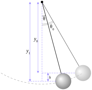 Figure 2. Trigonometry of a simple gravity pendulum. It can also be obtained via the conservation of mechanical energy principle: any object falling a vertical distance would acquire kinetic energy equal to that which it lost to the fall. In other words, gravitational potential energy is converted into kinetic energy. Change in potential energy is given by The change in kinetic energy (body started from rest) is given by Since no energy is lost, the gain in one must be equal to the loss in the other The change in velocity for a given change in height can be expressed as Using the arc length formula above, this equation can be rewritten in terms of dθ/dt: where h is the vertical distance the pendulum fell. Look at Figure 2, which presents the trigonometry of a simple pendulum. If the pendulum starts its swing from some initial angle θ0, then y0, the vertical distance from the screw, is given by Similarly, for y1, we have Then h is the difference of the two In terms of dθ/dt gives
This equation is known as the first integral of motion, it gives the velocity in terms of the location and includes an integration constant related to the initial displacement (θ0). We can differentiate, by applying the chain rule, with respect to time to get the acceleration which is the same result as obtained through force analysis. |


Small-angle approximation
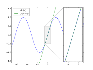
The differential equation given above is not easily solved, and there is no solution that can be written in terms of elementary functions. However, adding a restriction to the size of the oscillation's amplitude gives a form whose solution can be easily obtained. If it is assumed that the angle is much less than 1 radian (often cited as less than 0.1 radians, about 6°), or

then substituting for sin θ into Eq. 1 using the small-angle approximation,

yields the equation for a harmonic oscillator,

The error due to the approximation is of order θ3 (from Taylor expansion for sin θ).
Given the initial conditions θ(0) = θ0 and dθ/dt(0) = 0, the solution becomes

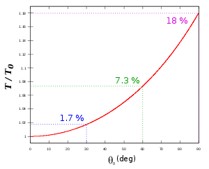
The motion is simple harmonic motion where θ0 is the amplitude of the oscillation (that is, the maximum angle between the rod of the pendulum and the vertical). The period of the motion, the time for a complete oscillation (outward and return) is

which is known as Christiaan Huygens's law for the period. Note that under the small-angle approximation, the period is independent of the amplitude θ0; this is the property of isochronism that Galileo discovered.
Rule of thumb for pendulum length
- can be expressed as


If SI units are used (i.e. measure in metres and seconds), and assuming the measurement is taking place on the Earth's surface, then g ≈ 9.81 m/s2, and g/π2 ≈ 1 (0.994 is the approximation to 3 decimal places).
Therefore, a relatively reasonable approximation for the length and period are,

where T0 is the number of seconds between two beats (one beat for each side of the swing), and l is measured in metres.
Arbitrary-amplitude period
For amplitudes beyond the small angle approximation, one can compute the exact period by first inverting the equation for the angular velocity obtained from the energy method (Eq. 2),

and then integrating over one complete cycle,

or twice the half-cycle

or four times the quarter-cycle

which leads to

Note that this integral diverges as θ0 approaches the vertical

so that a pendulum with just the right energy to go vertical will never actually get there. (Conversely, a pendulum close to its maximum can take an arbitrarily long time to fall down.)
This integral can be rewritten in terms of elliptic integrals as

where F is the incomplete elliptic integral of the first kind defined by

Or more concisely by the substitution

expressing θ in terms of u,
Eq. 3

Here K is the complete elliptic integral of the first kind defined by

For comparison of the approximation to the full solution, consider the period of a pendulum of length 1 m on Earth (g = 9.80665 m/s2) at initial angle 10 degrees is

The linear approximation gives

The difference between the two values, less than 0.2%, is much less than that caused by the variation of g with geographical location.
From here there are many ways to proceed to calculate the elliptic integral.
Legendre polynomial solution for the elliptic integral
Given Eq. 3 and the Legendre polynomial solution for the elliptic integral:

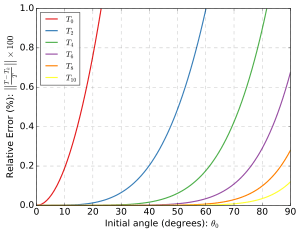
where n!! denotes the double factorial, an exact solution to the period of a pendulum is:

Figure 4 shows the relative errors using the power series. T0 is the linear approximation, and T2 to T10 include respectively the terms up to the 2nd to the 10th powers.
Power series solution for the elliptic integral
Another formulation of the above solution can be found if the following Maclaurin series:

is used in the Legendre polynomial solution above. The resulting power series is:[5]
- ,

Arithmetic-geometric mean solution for elliptic integral
Given Eq. 3 and the arithmetic–geometric mean solution of the elliptic integral:

where M(x,y) is the arithmetic-geometric mean of x and y.
This yields an alternative and faster-converging formula for the period:[6][7][8]

The first iteration of this algorithm gives

This approximation has the relative error of less than 1% for angles up to 96.11 degrees.[6] Since the expression can be written more concisely as


The second order expansion of reduces to


A second iteration of this algorithm gives

This second approximation has a relative error of less than 1% for angles up to 163.10 degrees.[6]
Approximate formulae for the nonlinear pendulum period
Though the exact period can be determined, for any finite amplitude rad, by evaluating the corresponding complete elliptic integral , where , this is often avoided in applications because it is not possible to express this integral in a closed form in terms of elementary functions. This has made way for research on simple approximate formulae for the increase of the pendulum period with amplitude (useful in introductory physics labs, classical mechanics, electromagnetism, acoustics, electronics, superconductivity, etc.[9] The approximate formulae found by different authors can be classified as follows:


- ‘Not so large-angle’ formulae, i.e. those yielding good estimates for amplitudes below rad (a natural limit for a bob on the end of a flexible string), though the deviation

with respect to the exact period increases monotonically with amplitude, being unsuitable for amplitudes near to rad. One of the simplest formulae found in literature is the following one by Lima (2006): , where .[10]


- ‘Very large-angle’ formulae, i.e. those which approximate the exact period asymptotically for amplitudes near to rad, with an error that increases monotonically for smaller
amplitudes (i.e., unsuitable for small amplitudes). One of the better such formulae is that by Cromer, namely:[11] .

Of course, the increase of with amplitude is more apparent when , as has been observed in many experiments using either a rigid rod or a disc.[12] As accurate timers and sensors are currently available even in introductory physics labs, the experimental errors found in ‘very large-angle’ experiments are already small enough for a comparison with the exact period and a very good agreement between theory and experiments in which friction is negligible has been found. Since this activity has been encouraged by many instructors, a simple approximate formula for the pendulum period valid for all possible amplitudes, to which experimental data could be compared, was sought. In 2008, Lima derived a weighted-average formula with this characteristic:[9]

,

where , which presents a maximum error of only 0.6% (at ).


Arbitrary-amplitude angular displacement Fourier series
The Fourier series expansion of is given by


where is the elliptic nome, , and the angular frequency. If one defines


can be approximated using the expansion

(see OEIS: A002103). Note that for we have , thus the approximation is applicable even for large amplitudes.

Examples
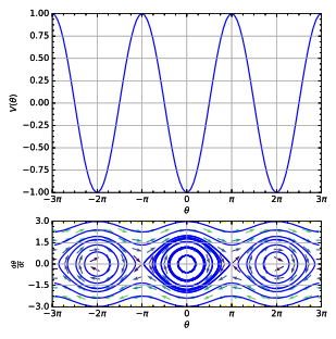
The animations below depict the motion of a simple (frictionless) pendulum with increasing amounts of initial displacement of the bob, or equivalently increasing initial velocity. The small graph above each pendulum is the corresponding phase plane diagram; the horizontal axis is displacement and the vertical axis is velocity. With a large enough initial velocity the pendulum does not oscillate back and forth but rotates completely around the pivot.
 Initial angle of 0°, a stable equilibrium
 Initial angle of 45°
 Initial angle of 90°
 Initial angle of 135°
 Initial angle of 170°
 Initial angle of 180°, unstable equilibrium
 Pendulum with just barely enough energy for a full swing
 Pendulum with enough energy for a full swing
Compound pendulum
A compound pendulum (or physical pendulum) is one where the rod is not massless, and may have extended size; that is, an arbitrarily shaped rigid body swinging by a pivot. In this case the pendulum's period depends on its moment of inertia I around the pivot point.
The equation of torque gives:

where:
- α is the angular acceleration.
- τ is the torque
The torque is generated by gravity so:

where:
- m is the mass of the body
- L is the distance from the pivot to the object's center of mass
- θ is the angle from the vertical
Hence, under the small-angle approximation sin θ ≈ θ,

where I is the moment of inertia of the body about the pivot point.
The expression for α is of the same form as the conventional simple pendulum and gives a period of[2]

And a frequency of

If the initial angle is taken into consideration (for large amplitudes), then the expression for becomes:


and gives a period of:

where θ0 is the maximum angle of oscillation (with respect to the vertical) and K(k) is the complete elliptic integral of the first kind.
Physical interpretation of the imaginary period
The Jacobian elliptic function that expresses the position of a pendulum as a function of time is a doubly periodic function with a real period and an imaginary period. The real period is, of course, the time it takes the pendulum to go through one full cycle. Paul Appell pointed out a physical interpretation of the imaginary period:[13] if θ0 is the maximum angle of one pendulum and 180° − θ0 is the maximum angle of another, then the real period of each is the magnitude of the imaginary period of the other.
Coupled pendulums
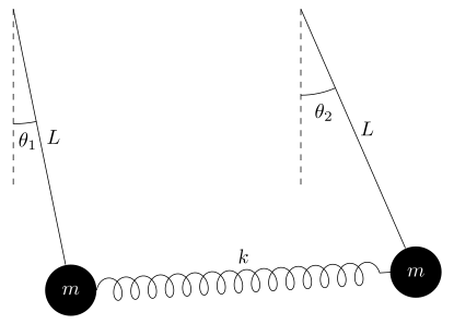
Coupled pendulums can affect each other's motion, either through a direction connection (such as a spring connecting the bobs) or through motions in a supporting structure (such as a tabletop). The equations of motion for two identical simple pendulums coupled by a spring connecting the bobs can be obtained using Lagrangian Mechanics.
The kinetic energy of the system is:

where is the mass of the bobs, is the length of the strings, and , are the angular displacements of the two bobs from equilibrium.


The potential energy of the system is:

where is the gravitational acceleration, and is the spring constant. The displacement of the spring from its equilibrium position assumes the small angle approximation.


The Lagrangian is then

which leads to the following set of coupled differential equations:

Adding and subtracting these two equations in turn, and applying the small angle approximation, gives two harmonic oscillator equations in the variables and :


with the corresponding solutions

where

and , , , are constants of integration.


Expressing the solutions in terms of and alone:

If the bobs are not given an initial push, then the condition requires , which gives (after some rearranging):


See also
- Blackburn pendulum
- Conical pendulum
- Cycloidal pendulum
- Double pendulum
- Inverted pendulum
- Kapitza's pendulum
- Spring pendulum
- Mathieu function
- Pendulum equations (software)
References
- defined by Christiaan Huygens: Huygens, Christian (1673). "Horologium Oscillatorium" (PDF). 17centurymaths. 17thcenturymaths.com. Retrieved 2009-03-01., Part 4, Definition 3, translated July 2007 by Ian Bruce
- Nave, Carl R. (2006). "Simple pendulum". Hyperphysics. Georgia State Univ. Retrieved 2008-12-10.
- Xue, Linwei (2007). "Pendulum Systems". Seeing and Touching Structural Concepts. Civil Engineering Dept., Univ. of Manchester, UK. Retrieved 2008-12-10.
- Weisstein, Eric W. (2007). "Simple Pendulum". Eric Weisstein's world of science. Wolfram Research. Retrieved 2009-03-09.
- Nelson, Robert; M. G. Olsson (February 1986). "The pendulum — Rich physics from a simple system". American Journal of Physics. 54 (2): 112–121. Bibcode:1986AmJPh..54..112N. doi:10.1119/1.14703.
- Carvalhaes, Claudio G.; Suppes, Patrick (December 2008), "Approximations for the period of the simple pendulum based on the arithmetic-geometric mean" (PDF), Am. J. Phys., 76 (12͒): 1150–1154, Bibcode:2008AmJPh..76.1150C, doi:10.1119/1.2968864, ISSN 0002-9505, retrieved 2013-12-14
- Borwein, J.M.; Borwein, P.B. (1987). Pi and the AGM. New York: Wiley. pp. 1–15. ISBN 0-471-83138-7. MR 0877728.
- Van Baak, Tom (November 2013). "A New and Wonderful Pendulum Period Equation" (PDF). Horological Science Newsletter. 2013 (5): 22–30.
- Lima, F. M. S. (2008-09-10). "Simple 'log formulae' for pendulum motion valid for any amplitude". European Journal of Physics. 29 (5): 1091–1098. doi:10.1088/0143-0807/29/5/021. ISSN 0143-0807 – via IoP journals.
- Lima, F. M. S.; Arun, P. (October 2006). "An accurate formula for the period of a simple pendulum oscillating beyond the small angle regime". American Journal of Physics. 74 (10): 892–895. arXiv:physics/0510206. Bibcode:2006AmJPh..74..892L. doi:10.1119/1.2215616. ISSN 0002-9505.
- Cromer, Alan (February 1995). "Many oscillations of a rigid rod". American Journal of Physics. 63 (2): 112–121. Bibcode:1995AmJPh..63..112C. doi:10.1119/1.17966. ISSN 0002-9505.
- Gil, Salvador; Legarreta, Andrés E.; Di Gregorio, Daniel E. (September 2008). "Measuring anharmonicity in a large amplitude pendulum". American Journal of Physics. 76 (9): 843–847. Bibcode:2008AmJPh..76..843G. doi:10.1119/1.2908184. ISSN 0002-9505.
- Appell, Paul (July 1878). "Sur une interprétation des valeurs imaginaires du temps en Mécanique" [On an interpretation of imaginary time values in mechanics]. Comptes Rendus Hebdomadaires des Séances de l'Académie des Sciences. 87 (1).
Further reading
- Baker, Gregory L.; Blackburn, James A. (2005). The Pendulum: A Physics Case Study (PDF). Oxford University Press.
- Ochs, Karlheinz (2011). "A comprehensive analytical solution of the nonlinear pendulum". European Journal of Physics. 32 (2): 479–490. Bibcode:2011EJPh...32..479O. doi:10.1088/0143-0807/32/2/019.
- Sala, Kenneth L. (1989). "Transformations of the Jacobian Amplitude Function and its Calculation via the Arithmetic-Geometric Mean". SIAM J. Math. Anal. 20 (6): 1514–1528. doi:10.1137/0520100.