Newton's method in optimization

The central problem of optimization is minimization of functions. Let us first consider the case of univariate functions, i.e., functions of a single real variable. We will later consider the more general and more practically useful multivariate case.

Given a twice differentiable function ${\displaystyle f:\mathbb {R} \to \mathbb {R} }$, we seek to solve the optimization problem

${\displaystyle \min _{x\in \mathbb {R} }f(x).}$

Newton's method attempts to solve this problem by constructing a sequence ${\displaystyle \{x_{k}\}}$ from an initial guess (starting point) ${\displaystyle x_{0}\in \mathbb {R} }$ that converges towards a minimizer ${\displaystyle x_{*}}$ of ${\displaystyle f}$ by using a sequence of second-order Taylor approximations of ${\displaystyle f}$ around the iterates. The second-order Taylor expansion of f around ${\displaystyle x_{k}}$ is

${\displaystyle f(x_{k}+t)\approx f(x_{k})+f'(x_{k})t+{\frac {1}{2}}f''(x_{k})t^{2}.}$

The next iterate ${\displaystyle x_{k+1}}$ is defined so as to minimize this quadratic approximation in ${\displaystyle t}$, and setting ${\displaystyle x_{k+1}=x_{k}+t}$. If the second derivative is positive, the quadratic approximation is a convex function of ${\displaystyle t}$, and its minimum can be found by setting the derivative to zero. Since

${\displaystyle \displaystyle 0={\frac {\rm {d}}{{\rm {d}}t}}\left(f(x_{k})+f'(x_{k})t+{\frac {1}{2}}f''(x_{k})t^{2}\right)=f'(x_{k})+f''(x_{k})t,}$

the minimum is achieved for

${\displaystyle t=-{\frac {f'(x_{k})}{f''(x_{k})}}.}$

Putting everything together, Newton's method performs the iteration

${\displaystyle x_{k+1}=x_{k}+t=x_{k}-{\frac {f'(x_{k})}{f''(x_{k})}}.}$

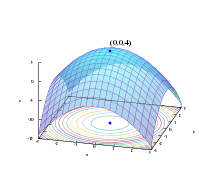
The geometric interpretation of Newton's method is that at each iteration, it amounts to the fitting of a paraboloid to the surface of ${\displaystyle f(x)}$ at the trial value ${\displaystyle x_{k}}$, having the same slopes and curvature as the surface at that point, and then proceeding to the maximum or minimum of that paraboloid (in higher dimensions, this may also be a saddle point).[2] Note that if ${\displaystyle f}$ happens to be a quadratic function, then the exact extremum is found in one step.

The above iterative scheme can be generalized to ${\displaystyle d}$ dimensions by replacing the derivative with the gradient (different authors use different notation for the gradient, including ${\displaystyle f'(x)=\nabla f(x)=g_{f}(x)\in \mathbb {R} ^{d}}$), and the reciprocal of the second derivative with the inverse of the Hessian matrix (different authors use different notation for the Hessian, including ${\displaystyle f''(x)=\nabla ^{2}f(x)=H_{f}(x)\in \mathbb {R} ^{d\times d}}$). One thus obtains the iterative scheme

${\displaystyle x_{k+1}=x_{k}-[f''(x_{k})]^{-1}f'(x_{k}),\qquad k\geq 0.}$

Often Newton's method is modified to include a small step size ${\displaystyle 0<\gamma \leq 1}$ instead of ${\displaystyle \gamma =1}$:

${\displaystyle x_{k+1}=x_{k}-\gamma [f''(x_{k})]^{-1}f'(x_{k}).}$

This is often done to ensure that the Wolfe conditions are satisfied at each step of the method. For step sizes other than 1, the method is often referred to as the relaxed or damped Newton's method.

If f is a strongly convex function with Lipschitz Hessian, then provided that ${\displaystyle x_{0}}$ is close enough to ${\displaystyle x_{*}=\arg \min f(x)}$, the sequence ${\displaystyle x_{0},x_{1},x_{2},\dots }$ generated by Newton's method will converge to the (necessarily unique) minimizer ${\displaystyle x_{*}}$ of ${\displaystyle f}$ quadratically fast. That is,

${\displaystyle \|x_{k+1}-x_{*}\|\leq {\frac {1}{2}}\|x_{k}-x_{*}\|^{2},\qquad \forall k\geq 0.}$

Finding the inverse of the Hessian in high dimensions to compute the Newton direction ${\displaystyle h=-(f''(x_{k}))^{-1}f'(x_{k})}$ can be an expensive operation. In such cases, instead of directly inverting the Hessian, it's better to calculate the vector ${\displaystyle h}$ as the solution to the system of linear equations

${\displaystyle [f''(x_{k})]h=-f'(x_{k})}$

which may be solved by various factorizations or approximately (but to great accuracy) using iterative methods. Many of these methods are only applicable to certain types of equations, for example the Cholesky factorization and conjugate gradient will only work if ${\displaystyle f''(x_{k})}$ is a positive definite matrix. While this may seem like a limitation, it's often a useful indicator of something gone wrong; for example if a minimization problem is being approached and ${\displaystyle f''(x_{k})}$ is not positive definite, then the iterations are converging to a saddle point and not a minimum.

On the other hand, if a constrained optimization is done (for example, with Lagrange multipliers), the problem may become one of saddle point finding, in which case the Hessian will be symmetric indefinite and the solution of ${\displaystyle x_{k+1}}$ will need to be done with a method that will work for such, such as the ${\displaystyle LDL^{\top }}$ variant of Cholesky factorization or the conjugate residual method.

There also exist various quasi-Newton methods, where an approximation for the Hessian (or its inverse directly) is built up from changes in the gradient.

If the Hessian is close to a non-invertible matrix, the inverted Hessian can be numerically unstable and the solution may diverge. In this case, certain workarounds have been tried in the past, which have varied success with certain problems. One can, for example, modify the Hessian by adding a correction matrix ${\displaystyle B_{k}}$ so as to make ${\displaystyle f''(x_{k})+B_{k}}$ positive definite. One approach is to diagonalize the Hessian and choose ${\displaystyle B_{k}}$ so that ${\displaystyle f''(x_{k})+B_{k}}$ has the same eigenvectors as the Hessian, but with each negative eigenvalue replaced by ${\displaystyle \epsilon >0}$.

An approach exploited in the Levenberg–Marquardt algorithm (which uses an approximate Hessian) is to add a scaled identity matrix to the Hessian, ${\displaystyle \mu I}$, with the scale adjusted at every iteration as needed. For large ${\displaystyle \mu }$ and small Hessian, the iterations will behave like gradient descent with step size ${\displaystyle 1/\mu }$. This results in slower but more reliable convergence where the Hessian doesn't provide useful information.

Many practical optimization problems, and especially those arising in data science and machine learning, involve a function ${\displaystyle f:\mathbb {R} ^{d}\to \mathbb {R} }$ which arises as an average of a very large number of simpler functions ${\displaystyle f_{i}}$:

${\displaystyle f(x)={\frac {1}{n}}\sum _{i=1}^{n}f_{i}(x).}$

In supervised machine learning, ${\displaystyle f_{i}(x)}$ represents the loss of model parameterized by vector ${\displaystyle x\in \mathbb {R} ^{d}}$ on data training point ${\displaystyle i}$, and ${\displaystyle f(x)}$ thus reflects the average loss of the model on the training data set. Problems of this type include linear least squares, logistic regression and deep neural network training.

In this situation, Newton's method for minimizing ${\displaystyle f}$ takes the form

${\displaystyle x_{k+1}=x_{k}-\left({\frac {1}{n}}\sum _{i=1}^{n}f''_{i}(x_{k})\right)^{-1}\left({\frac {1}{n}}\sum _{i=1}^{n}f_{i}'(x_{k})\right).}$

Recall that the key difficulty of standard Newton's method is the computation of Newton's step which is typically much more computationally demanding than the computation of the Hessian ${\displaystyle f''(x_{k})}$ and the gradient ${\displaystyle f'(x_{k})}$. However, in the setting considered here with ${\displaystyle f}$ being the sum of a very large number of functions, the situation reverses and the computation of ${\displaystyle f''(x_{k})}$ and ${\displaystyle f'(x_{k})}$ by averaging the Hessians and gradients of the individual functions ${\displaystyle f_{i}}$ becomes the bottleneck.

In this big ${\displaystyle n}$ regime, the above issue can be resolved by considering the stochastic Newton (SN) method developed and analyzed by Kovalev, Mishchenko and Richtárik.[3] SN is a generalization of Newton's method which allows for a flexible choice of the set ${\displaystyle S_{k}}$ of functions for which the computation of the Hessian and gradient is necessary. This set can be chosen to be ${\displaystyle S_{k}=\{1,2,\dots ,n\}}$, in which case SN reduces to Newton's method. However, one can also choose ${\displaystyle S_{k}=\{i\}}$, where ${\displaystyle i}$ is a random element of ${\displaystyle \{1,2,\dots ,n\}}$.

The Method. In general, SN is a parametric family of methods with parameter ${\displaystyle \tau \in \{1,2,\dots ,n\}}$ controlling the batch size. Given ${\displaystyle \tau }$, in iteration ${\displaystyle k}$ we let ${\displaystyle S_{k}}$ be a random subset of ${\displaystyle \{1,2,\dots ,n\}}$ chosen uniformly from all subsets of cardinality ${\displaystyle \tau }$. That is, all subsets of cardinality ${\displaystyle \tau }$ are chosen with probability ${\displaystyle 1/{d \choose \tau }}$. The two cases described above are special cases of this for ${\displaystyle \tau =n}$ and ${\displaystyle \tau =1}$, respectively.

The Stochastic Newton method maintains a sequence of vectors ${\displaystyle x_{k}^{1},x_{k}^{2},\cdots ,x_{k}^{n}\in \mathbb {R} ^{d}}$ for ${\displaystyle k\geq 0}$. At the beginning, i.e., for ${\displaystyle k=0}$, these vectors are initialized arbitrarily. A sensible choice is to set them to be equal. The method then performs the following steps:

${\displaystyle Step\;1:\quad x_{k+1}=\left({\frac {1}{n}}\sum _{i=1}^{n}f''_{i}(x_{k}^{i})\right)^{-1}\left({\frac {1}{n}}\sum _{i=1}^{n}f''_{i}(x_{k}^{i})x_{k}^{i}-f_{i}'(x_{k}^{i})\right)}$

${\displaystyle Step\;2:\quad {\text{Sample }}S_{k}\subseteq \{1,2,\dots ,n\}}$

${\displaystyle Step\;3:\quad x_{k+1}^{i}={\begin{cases}x_{k+1}&i\in S_{k}\\x_{k}^{i}&i\notin S_{k}\end{cases}}.}$

Note that if ${\displaystyle x_{0}^{1}=x_{0}^{2}=\cdots =x_{0}^{n}}$ and ${\displaystyle \tau =n}$, SN reduces to Newton's method described above. However, in contrast with Newton's method, in iteration ${\displaystyle k}$, SN needs to compute the gradients and Hessians of functions ${\displaystyle f_{i}}$ for ${\displaystyle i\in S_{k}}$ only. In particular, the batch size ${\displaystyle \tau }$ can be chosen to be a constant, in which case the cost of each iteration of SN is independent of ${\displaystyle n}$.

Convergence. For ${\displaystyle \tau =n}$, SN has local quadratic convergence rate identical to Newton's method. For ${\displaystyle \tau <n}$, SN has a local linear convergence rate independent of the condition number. In particular, it was shown by Kovalev, Mishchenko and Richtárik that if ${\displaystyle f}$ is strongly convex and has Lipschitz Hessian, then as long as the initial iterates ${\displaystyle x_{0}^{1},x_{0}^{2},\cdots ,x_{0}^{n}}$ are sufficiently close to the (necessarily) unique minimizer ${\displaystyle x_{*}}$ of ${\displaystyle f}$, then

${\displaystyle {\rm {E}}\left[{\frac {1}{n}}\sum _{i=1}^{n}\|x_{k}^{i}-x_{*}\|^{2}\right]\leq \left(1-{\frac {3\tau }{4n}}\right)^{k}\left[{\frac {1}{n}}\sum _{i=1}^{n}\|x_{0}^{i}-x_{*}\|^{2}\right],}$

where ${\displaystyle {\rm {E}}[\cdot ]}$ refers to mathematical expectation with respect to the randomness inherent in the algorithm.

This is a much better rate than what is obtainable by any stochastic first order method, such as stochastic gradient descent. Indeed, the convergence rate of all first order method depends on the condition number of ${\displaystyle f}$, which is typically defined as ${\displaystyle \kappa =L/\mu }$, where ${\displaystyle 0<\mu \leq L}$ are constants such that

${\displaystyle \mu I\preceq f''(x)\preceq LI,\qquad \forall x\in \mathbb {R} ^{d}.}$

There are various techniques which can to some extent reduce but which can't completely eliminate the effect of the conditioning ${\displaystyle \kappa }$ on the convergence rate of first order methods. These techniques include adaptive stepsizes, minibatching, importance sampling, Polyak momentum, Nesterov's momentum and variance reduction. In contrast to all of these techniques, SN completely removes the effect of conditioning. However, as Newton's method, SN suffers from reliance on local convergence guarantees only.

• Quasi-Newton method
• Gradient descent
• Gauss–Newton algorithm
• Levenberg–Marquardt algorithm
• Trust region
• Optimization
• Nelder–Mead method

• Avriel, Mordecai (2003). Nonlinear Programming: Analysis and Methods. Dover Publishing. ISBN 0-486-43227-0.
• Bonnans, J. Frédéric; Gilbert, J. Charles; Lemaréchal, Claude; Sagastizábal, Claudia A. (2006). Numerical optimization: Theoretical and practical aspects. Universitext (Second revised ed. of translation of 1997 French ed.). Berlin: Springer-Verlag. doi:10.1007/978-3-540-35447-5. ISBN 3-540-35445-X. MR 2265882.
• Fletcher, Roger (1987). Practical Methods of Optimization (2nd ed.). New York: John Wiley & Sons. ISBN 978-0-471-91547-8.
• Givens, Geof H.; Hoeting, Jennifer A. (2013). Computational Statistics. Hoboken, New Jersey: John Wiley & Sons. pp. 24–58. ISBN 978-0-470-53331-4.
• Nocedal, Jorge; Wright, Stephen J. (1999). Numerical Optimization. Springer-Verlag. ISBN 0-387-98793-2.
• Kovalev, Dmitry; Mishchenko, Konstantin; Richtárik, Peter (2019). "Stochastic Newton and cubic Newton methods with simple local linear-quadratic rates". arXiv:1912.01597 [cs.LG].

• Korenblum, Daniel (Aug 29, 2015). "Newton-Raphson visualization (1D)". Bl.ocks. ffe9653768cb80dfc0da.