Gradient descent

Illustration of gradient descent on a series of level sets

Gradient descent is based on the observation that if the multi-variable function ${\displaystyle F(\mathbf {x} )}$ is defined and differentiable in a neighborhood of a point ${\displaystyle \mathbf {a} }$, then ${\displaystyle F(\mathbf {x} )}$ decreases fastest if one goes from ${\displaystyle \mathbf {a} }$ in the direction of the negative gradient of ${\displaystyle F}$ at ${\displaystyle \mathbf {a} ,-\nabla F(\mathbf {a} )}$. It follows that, if

${\displaystyle \mathbf {a} _{n+1}=\mathbf {a} _{n}-\gamma \nabla F(\mathbf {a} _{n})}$

for ${\displaystyle \gamma \in \mathbb {R} _{+}}$ small enough, then ${\displaystyle F(\mathbf {a_{n}} )\geq F(\mathbf {a_{n+1}} )}$. In other words, the term ${\displaystyle \gamma \nabla F(\mathbf {a} )}$ is subtracted from ${\displaystyle \mathbf {a} }$ because we want to move against the gradient, toward the local minimum. With this observation in mind, one starts with a guess ${\displaystyle \mathbf {x} _{0}}$ for a local minimum of ${\displaystyle F}$, and considers the sequence ${\displaystyle \mathbf {x} _{0},\mathbf {x} _{1},\mathbf {x} _{2},\ldots }$ such that

${\displaystyle \mathbf {x} _{n+1}=\mathbf {x} _{n}-\gamma _{n}\nabla F(\mathbf {x} _{n}),\ n\geq 0.}$

We have a monotonic sequence

${\displaystyle F(\mathbf {x} _{0})\geq F(\mathbf {x} _{1})\geq F(\mathbf {x} _{2})\geq \cdots ,}$

so hopefully the sequence ${\displaystyle (\mathbf {x} _{n})}$ converges to the desired local minimum. Note that the value of the step size ${\displaystyle \gamma }$ is allowed to change at every iteration. With certain assumptions on the function ${\displaystyle F}$ (for example, ${\displaystyle F}$ convex and ${\displaystyle \nabla F}$ Lipschitz) and particular choices of ${\displaystyle \gamma }$ (e.g., chosen either via a line search that satisfies the Wolfe conditions, or the Barzilai–Borwein method[3][4] shown as following),

${\displaystyle \gamma _{n}={\frac {\left|\left(\mathbf {x} _{n}-\mathbf {x} _{n-1}\right)^{T}\left[\nabla F(\mathbf {x} _{n})-\nabla F(\mathbf {x} _{n-1})\right]\right|}{\left\|\nabla F(\mathbf {x} _{n})-\nabla F(\mathbf {x} _{n-1})\right\|^{2}}}}$

convergence to a local minimum can be guaranteed. When the function ${\displaystyle F}$ is convex, all local minima are also global minima, so in this case gradient descent can converge to the global solution.

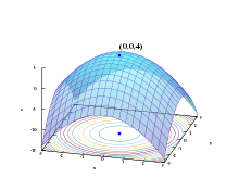
This process is illustrated in the adjacent picture. Here ${\displaystyle F}$ is assumed to be defined on the plane, and that its graph has a bowl shape. The blue curves are the contour lines, that is, the regions on which the value of ${\displaystyle F}$ is constant. A red arrow originating at a point shows the direction of the negative gradient at that point. Note that the (negative) gradient at a point is orthogonal to the contour line going through that point. We see that gradient descent leads us to the bottom of the bowl, that is, to the point where the value of the function ${\displaystyle F}$ is minimal.

An analogy for understanding gradient descent

Fog in the mountains

The basic intuition behind gradient descent can be illustrated by a hypothetical scenario. A person is stuck in the mountains and is trying to get down (i.e. trying to find the global minimum). There is heavy fog such that visibility is extremely low. Therefore, the path down the mountain is not visible, so they must use local information to find the minimum. They can use the method of gradient descent, which involves looking at the steepness of the hill at their current position, then proceeding in the direction with the steepest descent (i.e. downhill). If they were trying to find the top of the mountain (i.e. the maximum), then they would proceed in the direction of steepest ascent (i.e. uphill). Using this method, they would eventually find their way down the mountain or possibly get stuck in some hole (i.e. local minimum or saddle point), like a mountain lake. However, assume also that the steepness of the hill is not immediately obvious with simple observation, but rather it requires a sophisticated instrument to measure, which the person happens to have at the moment. It takes quite some time to measure the steepness of the hill with the instrument, thus they should minimize their use of the instrument if they wanted to get down the mountain before sunset. The difficulty then is choosing the frequency at which they should measure the steepness of the hill so not to go off track.

In this analogy, the person represents the algorithm, and the path taken down the mountain represents the sequence of parameter settings that the algorithm will explore. The steepness of the hill represents the slope of the error surface at that point. The instrument used to measure steepness is differentiation (the slope of the error surface can be calculated by taking the derivative of the squared error function at that point). The direction they choose to travel in aligns with the gradient of the error surface at that point. The amount of time they travel before taking another measurement is the learning rate of the algorithm. See Backpropagation § Limitations for a discussion of the limitations of this type of "hill descending" algorithm.

The steepest descent algorithm applied to the Wiener filter.[5]

Gradient descent can be used to solve a system of linear equations, reformulated as a quadratic minimization problem, e.g., using linear least squares. The solution of

${\displaystyle A\mathbf {x} -\mathbf {b} =0}$

in the sense of linear least squares is defined as minimizing the function

${\displaystyle F(\mathbf {x} )=\left\|A\mathbf {x} -\mathbf {b} \right\|^{2}.}$

In traditional linear least squares for real ${\displaystyle A}$ and ${\displaystyle \mathbf {b} }$ the Euclidean norm is used, in which case

${\displaystyle \nabla F(\mathbf {x} )=2A^{T}(A\mathbf {x} -\mathbf {b} ).}$

In this case, the line search minimization, finding the locally optimal step size ${\displaystyle \gamma }$ on every iteration, can be performed analytically, and explicit formulas for the locally optimal ${\displaystyle \gamma }$ are known.[6]

The algorithm is rarely used for solving linear equations, with the conjugate gradient method being one of the most popular alternatives. The number of gradient descent iterations is commonly proportional to the spectral condition number ${\displaystyle \kappa (A)}$ of the system matrix ${\displaystyle A}$ (the ratio of the maximum to minimum eigenvalues of ${\displaystyle A^{T}A}$), while the convergence of conjugate gradient methodis typically determined by a square root of the condition number, i.e., is much faster. Both methods can benefit from preconditioning, where gradient descent may require less assumptions on the preconditioner.[7]

Gradient descent can also be used to solve a system of nonlinear equations. Below is an example that shows how to use the gradient descent to solve for three unknown variables, x₁, x₂, and x₃. This example shows one iteration of the gradient descent.

Consider the nonlinear system of equations

${\displaystyle {\begin{cases}3x_{1}-\cos(x_{2}x_{3})-{\tfrac {3}{2}}=0\\4x_{1}^{2}-625x_{2}^{2}+2x_{2}-1=0\\\exp(-x_{1}x_{2})+20x_{3}+{\tfrac {10\pi -3}{3}}=0\end{cases}}}$

Let us introduce the associated function

${\displaystyle G(\mathbf {x} )={\begin{bmatrix}3x_{1}-\cos(x_{2}x_{3})-{\tfrac {3}{2}}\\4x_{1}^{2}-625x_{2}^{2}+2x_{2}-1\\\exp(-x_{1}x_{2})+20x_{3}+{\tfrac {10\pi -3}{3}}\\\end{bmatrix}},}$

where

${\displaystyle \mathbf {x} ={\begin{bmatrix}x_{1}\\x_{2}\\x_{3}\\\end{bmatrix}}.}$

One might now define the objective function

${\displaystyle F(\mathbf {x} )={\frac {1}{2}}G^{\mathrm {T} }(\mathbf {x} )G(\mathbf {x} )={\frac {1}{2}}\left[\left(3x_{1}-\cos(x_{2}x_{3})-{\frac {3}{2}}\right)^{2}+\left(4x_{1}^{2}-625x_{2}^{2}+2x_{2}-1\right)^{2}+\left(\exp(-x_{1}x_{2})+20x_{3}+{\frac {10\pi -3}{3}}\right)^{2}\right],}$

which we will attempt to minimize. As an initial guess, let us use

${\displaystyle \mathbf {x} ^{(0)}=\mathbf {0} ={\begin{bmatrix}0\\0\\0\\\end{bmatrix}}.}$

We know that

${\displaystyle \mathbf {x} ^{(1)}=\mathbf {0} -\gamma _{0}\nabla F(\mathbf {0} )=\mathbf {0} -\gamma _{0}J_{G}(\mathbf {0} )^{\mathrm {T} }G(\mathbf {0} ),}$

where the Jacobian matrix ${\displaystyle J_{G}}$ is given by

${\displaystyle J_{G}(\mathbf {x} )={\begin{bmatrix}3&\sin(x_{2}x_{3})x_{3}&\sin(x_{2}x_{3})x_{2}\\8x_{1}&-1250x_{2}+2&0\\-x_{2}\exp {(-x_{1}x_{2})}&-x_{1}\exp(-x_{1}x_{2})&20\\\end{bmatrix}}.}$

We calculate:

${\displaystyle J_{G}(\mathbf {0} )={\begin{bmatrix}3&0&0\\0&2&0\\0&0&20\end{bmatrix}},\qquad G(\mathbf {0} )={\begin{bmatrix}-2.5\\-1\\10.472\end{bmatrix}}.}$

Thus

${\displaystyle \mathbf {x} ^{(1)}=\mathbf {0} -\gamma _{0}{\begin{bmatrix}-7.5\\-2\\209.44\end{bmatrix}},}$

and

${\displaystyle F(\mathbf {0} )=0.5\left((-2.5)^{2}+(-1)^{2}+(10.472)^{2}\right)=58.456.}$

An animation showing the first 83 iterations of gradient descent applied to this example. Surfaces are isosurfaces of ${\displaystyle F(\mathbf {x} ^{(n)})}$ at current guess ${\displaystyle \mathbf {x} ^{(n)}}$, and arrows show the direction of descent. Due to a small and constant step size, the convergence is slow.

Now, a suitable ${\displaystyle \gamma _{0}}$ must be found such that

${\displaystyle F\left(\mathbf {x} ^{(1)}\right)\leq F\left(\mathbf {x} ^{(0)}\right)=F(\mathbf {0} ).}$

This can be done with any of a variety of line search algorithms. One might also simply guess ${\displaystyle \gamma _{0}=0.001,}$ which gives

${\displaystyle \mathbf {x} ^{(1)}={\begin{bmatrix}0.0075\\0.002\\-0.20944\\\end{bmatrix}}.}$

Evaluating the objective function at this value, yields

${\displaystyle F\left(\mathbf {x} ^{(1)}\right)=0.5\left((-2.48)^{2}+(-1.00)^{2}+(6.28)^{2}\right)=23.306.}$

The decrease from ${\displaystyle F(\mathbf {0} )=58.456}$ to the next step's value of

${\displaystyle F\left(\mathbf {x} ^{(1)}\right)=23.306}$

is a sizable decrease in the objective function. Further steps would reduce its value further, until an approximate solution to the system was found.

Gradient descent works in spaces of any number of dimensions, even in infinite-dimensional ones. In the latter case, the search space is typically a function space, and one calculates the Fréchet derivative of the functional to be minimized to determine the descent direction.[8]

That gradient descent works in any number of dimensions (finite number at least) can be seen as a consequence of the Cauchy-Schwarz inequality. In the article on that subject here on Wikipedia it’s proven that the magnitude of the inner (dot) product of two vectors of any dimension is maximized when the are colinear. In the case of gradient descent, that would be when the vector of independent variable adjustments is proportional to the gradient vector of partial derivatives.

The gradient descent can take many iterations to compute a local minimum with a required accuracy, if the curvature in different directions is very different for the given function. For such functions, preconditioning, which changes the geometry of the space to shape the function level sets like concentric circles, cures the slow convergence. Constructing and applying preconditioning can be computationally expensive, however.

The gradient descent can be combined with a line search, finding the locally optimal step size ${\displaystyle \gamma }$ on every iteration. Performing the line search can be time-consuming. Conversely, using a fixed small ${\displaystyle \gamma }$ can yield poor convergence.

Methods based on Newton's method and inversion of the Hessian using conjugate gradient techniques can be better alternatives.[9][10] Generally, such methods converge in fewer iterations, but the cost of each iteration is higher. An example is the BFGS method which consists in calculating on every step a matrix by which the gradient vector is multiplied to go into a "better" direction, combined with a more sophisticated line search algorithm, to find the "best" value of ${\displaystyle \gamma .}$ For extremely large problems, where the computer-memory issues dominate, a limited-memory method such as L-BFGS should be used instead of BFGS or the steepest descent.

Gradient descent can be viewed as applying Euler's method for solving ordinary differential equations ${\displaystyle x'(t)=-\nabla f(x(t))}$ to a gradient flow. In turn, this equation may be derived as an optimal controller[11] for the control system ${\displaystyle x'(t)=u(t)}$ with ${\displaystyle u(t)}$ given in feedback form ${\displaystyle u(t)=-\nabla f(x(t))}$.

The following code examples apply the gradient descent algorithm to find the minimum of the function ${\displaystyle f(x)=x^{4}-3x^{3}+2,}$ with derivative ${\displaystyle f'(x)=4x^{3}-9x^{2}.}$

Solving for ${\displaystyle 4x^{3}-9x^{2}=0}$ and evaluation of the second derivative at the solutions shows the function has a plateau point at 0 and a global minimum at ${\displaystyle x={\tfrac {9}{4}}.}$

x = 6  # Starting point
step_size = 0.01
step_tolerance = 0.00001
max_iterations = 10000

# Derivative function f'(x)
df = lambda x: 4 * x**3 - 9 * x ** 2

# Gradient descent iteration
for j in range(max_iterations):
    step = step_size * df(x)
    x -= step

    if abs(step) <= step_tolerance:
        break

print('Minimum:', x) # 2.2499646074278457
print('Exact:', 9/4) # 2.25
print('Iterations:',j) # 69

x = 6; (* Starting point *)
stepSize = 0.01;
stepTolerance = 0.0001;
maxIterations = 10000;

(* Function to find the minimum of *)
f[x_] := x^4 - 3 x^3 + 2;

(* Gradient descent iteration *)
For[j = 0, j < maxIterations, j++,
    step = stepSize * f'[x];
    x = x - step;
    If[Abs[step] < stepTolerance, Break[]]]
Print["Minimum: " <> ToString@x] (* 2.24966 *)
Print["Exact: " <> ToString@N@(9/4)] (* 2.25 *)
Print["Iterations: " <> ToString@j] (* 59 *)

import math._

val curX = 6
val gamma = 0.01 
val precision = 0.00001 
val previousStepSize = 1 / precision

def df(x: Double): Double = 4 * pow(x, 3) - 9 * pow(x, 2)

def gradientDescent(precision: Double, previousStepSize: Double, curX: Double): Double = {
  if (previousStepSize > precision) {
    val newX = curX + -gamma * df(curX)	
    println(curX)
    gradientDescent(precision, abs(newX - curX), newX)
  } else curX	 
}

val ans = gradientDescent(precision, previousStepSize, curX)
println(s"The local minimum occurs at $ans")

(defn df [x] (- (* 4 x x x) (* 9 x x)))

(defn gradient-descent [thresh iters gamma x df]
  (loop [prev-x x
         cur-x (- x (* gamma (df x)))
         iters iters]
    (if (or (< (Math/abs (- cur-x prev-x)) thresh)
            (zero? iters))
      cur-x
      (recur cur-x
             (- cur-x (* gamma (df cur-x)))
             (dec iters)))))

(prn "The minimum is found at: " (gradient-descent 0.00001 10000 0.01 6 df))

;; This will output: "The minimum is found at: " 2.2499646074278457

(defn gradient-descent [iters gamma x df]
  (reduce (fn [x _]
            (- x (* gamma (df x))))
          x
          (range iters)))

(prn "The minimum is found at: " (gradient-descent 10000 0.01 6 df))

;; This will output: "The minimum is found at: " 2.249999999999999

(defn gradient-descent [n-iters gamma x df]
  (nth (iterate (fn [x] (- x (* gamma (df x)))) x)
       n-iters))

(prn "The minimum is found at: " (gradient-descent 10000 0.01 6 df))

;; This will output: "The minimum is found at: " 2.249999999999999

 1 import java.util.function.Function;
 2 import static java.lang.Math.pow;
 3 import static java.lang.Math.abs;
 4 
 5 public class GradientDescent {
 6     static double gamma = 0.01;
 7     static double precision = 0.00001;
 8     
 9     public static void main(String[] args){
10         Function<Double, Double> df = x -> 4 * pow(x, 3) - 9 * pow(x, 2);
11         double res = gradientDescent(df);
12         System.out.println(String.format("The local minimum occurs at %f", res));
13     }
14 
15     static double gradientDescent (Function < Double, Double > f){
16 
17             double curX = 6.0;
18             double previousStepSize = 1.0;
19 
20             while (previousStepSize > precision) {
21                 double prevX = curX;
22                 curX -= gamma * f.apply(prevX);
23                 previousStepSize = abs(curX - prevX);
24             }
25             return curX;
26     }
27 }

import kotlin.math.abs
import kotlin.math.pow

val gradientDescent =
    { gamma: Double ->
        { precision: Double ->
            { initialStepSize: Double ->
                { function: (Double) -> Double ->
                    { x: Double ->
                        val seq = generateSequence(Pair(initialStepSize, x)) { p ->
                            (p.second - gamma * function(p.second)).let { newX ->
                                val newStepSize = abs(newX - p.second)
                                Pair(newStepSize, newX)
                            }
                        }
                        seq.first { p -> p.first < precision }.second
                    }
                }
            }
        }
    }

val standardGradientDescentComputer = gradientDescent(0.01)(0.00001)(1.0)

fun main() {
    val df: (Double) -> Double = { x ->  4 * x.pow(3) - 9 * x.pow(2) }
    val dfGradientDescent = standardGradientDescentComputer(df)
    val result = dfGradientDescent(6.0)
    println("The local minimum occurs at $result")
}

x = 6.0 # Starting point
step_size = 0.01
step_tolerance = 0.00001
max_iterations = 10000
iterations = 0

# Derivative function f'(x)
df(x) = 4x^3 - 9x^2

# Gradient descent iteration
for j = 1:max_iterations
    global x, iterations
    step = step_size*df(x)
    x -= step

    if abs(step) <= step_tolerance
        break
    end

    iterations += 1
end

println("Minimum: ", x) # 2.2499646074278457
println("Exact: ", 9/4) # 2.25
println("Iterations: ", iterations) # 69

#include <stdio.h>
#include <stdlib.h>

double dfx(double x) {
    return 4*(x*x*x) - 9*(x*x);
}

double abs_val(double x) {
    return x > 0 ? x : -x;
}

double gradient_descent(double dx, double error, double gamma, unsigned int max_iters) {
    double c_error = error + 1;
    unsigned int iters = 0;
    double p_error;
    while (error < c_error && iters < max_iters) {
        p_error = dx;
        dx -= dfx(p_error) * gamma;
	    c_error = abs_val(p_error-dx);
        printf("\nc_error %f\n", c_error);
        iters++;
    }
    return dx;
}

int main() {
    double dx = 6;
    double error = 1e-6;
    double gamma = 0.01;
    unsigned int max_iters = 10000;
    printf("The local minimum is: %f\n", gradient_descent(dx, error, gamma, max_iters));
    return 0;
}

const convergeGradientDescent = (
gradientFunction, // the gradient Function 
x0 = 0, // starting position
maxIters = 1000, // Maximum number of iterations
precision = 0.00001,  //  Desired precision of result
gamma = 0.01  // Step size multiplier
) => {
  let step = 2 * precision
  let iter = 0
  let x = x0
  while (true) {
    step = gamma * gradientFunction(x)
    x -= step
    iter++
    console.log(iter)
    if (iter > maxIters) throw Error("Exceeded maximum iterations")
    if (Math.abs(step) < precision) {
      console.log(`Minimum at: ${x}`)
      console.log(`After ${iter} iteration(s)`)
      return(x)
    }
  }
}

// TEST
// gradient function, df
const df = (x) => (4 * x - 9) * x * x
convergeGradientDescent(df,6)
//2.2499646074278457
//Minimum at: 2.2499646074278457
//after 70 iteration(s)

// adjust training set size

const M = 10;

// generate random training set

const DATA = [];

const getRandomIntFromInterval = (min, max) =>
  Math.floor(Math.random() * (max - min + 1) + min);

const createRandomPortlandHouse = () => ({
  squareMeter: getRandomIntFromInterval(0, 100),
  price: getRandomIntFromInterval(0, 100),
});

for (let i = 0; i < M; i++) {
  DATA.push(createRandomPortlandHouse());
}

const _x = DATA.map(date => date.squareMeter);
const _y = DATA.map(date => date.price);

// linear regression and gradient descent

const LEARNING_RATE = 0.0003;

let thetaOne = 0;
let thetaZero = 0;

const hypothesis = x => thetaZero + thetaOne * x;

const learn = (x, y, alpha) => {
  let thetaZeroSum = 0;
  let thetaOneSum = 0;

  for (let i = 0; i < M; i++) {
    thetaZeroSum += hypothesis(x[i]) - y[i];
    thetaOneSum += (hypothesis(x[i]) - y[i]) * x[i];
  }

  thetaZero = thetaZero - (alpha / M) * thetaZeroSum;
  thetaOne = thetaOne - (alpha / M) * thetaOneSum;
}

const MAX_ITER = 1500;
for (let i = 0; i < MAX_ITER; i++) {
  learn(_x, _y, LEARNING_RATE);
  console.log('thetaZero ', thetaZero, 'thetaOne', thetaOne);
}

x = 6.0; % Starting point
step_size = 0.01;
step_tolerance = 0.00001;
max_iterations = 10000;

% Derivative function f'(x)
df = @(x) 4*x^3 - 9*x^2;

% Gradient descent iteration
for j = 0:max_iterations
    step = step_size*df(x);
    x = x - step;

    if abs(step) <= step_tolerance
        break
    end
end

fprintf('Minimum: %.6f\n', x); % 2.249965
fprintf('Exact: %.6f\n', 9/4); % 2.250000
fprintf('Iterations: %d\n', j); % 69

x = [0 0 0]'; % Starting point
step_size = 0.001;
max_iterations = 10000;
function_tolerance = 0.01;
step_tolerance = 0.001;

% Multi-variate vector-valued function G(x)
G = @(x) [
    3*x(1) - cos(x(2)*x(3)) - 3/2           ;
    4*x(1)^2 - 625*x(2)^2 + 2*x(2) - 1      ;
    exp(-x(1)*x(2)) + 20*x(3) + (10*pi-3)/3];

% Jacobian of G
JG = @(x) [
    3,                     sin(x(2)*x(3))*x(3),   sin(x(2)*x(3))*x(2) ;
    8*x(1),                -1250*x(2)+2,          0                   ;
    -x(2)*exp(-x(1)*x(2)), -x(1)*exp(-x(1)*x(2)), 20                 ];

% Objective function F(x) to minimize in order to solve G(x)=0
F = @(x) 0.5*G(x)'*G(x);

% Gradient of F (partial derivatives)
dF = @(x) JG(x)'*G(x);

% Print progress
prog_format = 'j:%03d | x:[% .3f,% .3f,% .3f] | F(x):%f\n';
prog = @(j,x) fprintf(prog_format, j, x, F(x));

% Gradient descent iteration
fvals = F(x);
steps = max(abs(step_size * dF(x)));
prog(0,x);
for j = 1:max_iterations
    step = step_size * dF(x);
    x = x - step;
    fval = F(x);
    
    % Log function value and step size
    fvals(end+1) = fval;
    steps(end+1) = max(abs(step));
    
    prog(j,x); % Display progress

    if fvals(end) < function_tolerance
        fprintf('Function value smaller than ''function_tolerance''\n')
        break
    end
    
    if max(abs(step)) < step_tolerance
        fprintf('Step size smaller than ''step_tolerance''\n')
        break
    end
end

% Plot
figure(1); clf;
yyaxis left; semilogy(0:j,fvals); ylabel('Function value');
yyaxis right; semilogy(0:j,steps); ylabel('Step size');
grid on; xlim([0 j+1]); xlabel('Iteration');

% Higher quality solution (fminsearch(F,[0 0 0]'))
better_x = [1004/1205 -187/3614 -265/504];

% Evaluate final solution
fprintf('Minimum x:    [% .6f,% .6f,% .6f]\n',x);
fprintf('Better x:     [% .6f,% .6f,% .6f]\n',better_x);
fprintf('Minimum G(x): [% .6f,% .6f,% .6f]\n',G(x));
fprintf('Exact G(x):   [% .6f,% .6f,% .6f]\n',[0,0,0]);

% Output:
%
% j:000 | x:[ 0.000, 0.000, 0.000] | F(x):58.456136
% j:001 | x:[ 0.007, 0.002,-0.209] | F(x):23.306394
% j:002 | x:[ 0.015, 0.002,-0.335] | F(x):10.617030
% ...
% j:218 | x:[ 0.721, 0.043,-0.522] | F(x):0.057119
% j:219 | x:[ 0.722, 0.043,-0.522] | F(x):0.056107
% j:220 | x:[ 0.723, 0.043,-0.522] | F(x):0.055113
% Step size smaller than 'step_tolerance'
% Minimum x:    [ 0.722583, 0.043324,-0.522074]
% Better x:     [ 0.833195,-0.051743,-0.525794]
% Minimum G(x): [-0.331996, 0.002029,-0.000318]
% Exact G(x):   [ 0.000000, 0.000000, 0.000000]

# set up a stepsize multiplier
gamma = 0.003

# set up a number of iterations
iter = 500

# define the objective function f(x) = x^4 - 3*x^3 + 2
objFun = function(x) return(x^4 - 3*x^3 + 2)

# define the gradient of f(x) = x^4 - 3*x^3 + 2
gradient = function(x) return((4*x^3) - (9*x^2))

# randomly initialize a value to x
set.seed(100)
x = floor(runif(1, 0, 10))

# create a vector to contain all xs for all steps
x.All = numeric(iter)

# gradient descent method to find the minimum
for(i in seq_len(iter)){
        x = x - gamma*gradient(x)
        x.All[i] = x
        print(x)
}

# print result and plot all xs for every iteration
print(paste("The minimum of f(x) is ", objFun(x), " at position x = ", x, sep = ""))
plot(x.All, type = "l")

fn derivative(x: &f32) -> f32 {
    4.0 * x.powf(3.0) - 9.0 * x.powf(2.0)
}

fn main() {
    let mut next_x: f32 = 6.0; // We start the search at x=6
    let step_size: f32 = 0.01;
    let precision: f32 = 0.00001;
    let max_iterations: i32 = 10000;

    for i in 0..max_iterations {
        let current_x = next_x;
        next_x = current_x - step_size * derivative(&current_x);

        let step = next_x - current_x;
        println!("iteration: {}, current x: {}, step: {}", i, current_x, step);
        if step.abs() <= precision {
            break;
        }
    }
}

df :: Double -> Double
df x = 4 * x ** 3 - 9 * x ** 2

gradientDescent :: Double -> Double -> Double -> Double -> IO Double
gradientDescent gamma precision previousStepSize curX =
  if previousStepSize > precision
    then do
      let newX = curX - (gamma * df curX)
      print curX
      gradientDescent gamma precision (abs (newX - curX)) newX
    else return curX

runGradientDescent :: IO Double
runGradientDescent = gradientDescent gamma precision previousStepSize curX
 where
  curX             = 6
  gamma            = 0.01
  precision        = 0.0001
  previousStepSize = 1 / precision

package main

import (
	"fmt"
	"math"
)

//Derivative function
func derivatedFunction(f func(float64) float64) func(float64) float64 {
	h := 0.000001
	return func(x float64) float64 {
		return (f(x+h) - f(x-h)) / (2 * h)
	}
}

func f(x float64) float64 {
	return (math.Pow(x, 4) - 3*math.Pow(x, 3) + 2)
}

func gradientDescendent() float64 {
	var (
		next_x    = 1.00      // We start the search at x = 1
		gamma     = 0.01      // Step size multiplier
		precision = 0.0000001 // Desired precision of result
		max_iters = 100000    // Maximum number of iterations
	)
	var current_x, step float64
	var i int
	df := derivatedFunction(f)

	for i = 0; i < max_iters; i++ {
		current_x = next_x
		next_x = current_x - gamma*df(current_x)
		step = next_x - current_x
		if math.Abs(step) <= precision {
			break
		}

	}
	return next_x
	//"Minimum at 2.2499646074278457"
}

func main() {
	minimunAt := gradientDescendent()
	fmt.Printf("Minimum at %.8f\n", minimunAt)
}

Gradient descent can be extended to handle constraints by including a projection onto the set of constraints. This method is only feasible when the projection is efficiently computable on a computer. Under suitable assumptions, this method converges. This method is a specific case of the forward-backward algorithm for monotone inclusions (which includes convex programming and variational inequalities).[13]

• Boyd, Stephen; Vandenberghe, Lieven (2004). "Unconstrained Minimization" (PDF). Convex Optimization. New York: Cambridge University Press. pp. 457–520. ISBN 0-521-83378-7.

• Using gradient descent in C++, Boost, Ublas for linear regression
• Series of Khan Academy videos discusses gradient ascent
• Online book teaching gradient descent in deep neural network context
• "Gradient Descent, How Neural Networks Learn". 3Blue1Brown. October 16, 2017 – via YouTube.

References

- Lemaréchal, C. (2012). "Cauchy and the Gradient Method" (PDF). Doc Math Extra: 251–254.
- Curry, Haskell B. (1944). "The Method of Steepest Descent for Non-linear Minimization Problems". Quart. Appl. Math. 2 (3): 258–261. doi:10.1090/qam/10667.
- Barzilai, Jonathan; Borwein, Jonathan M. (1988). "Two-Point Step Size Gradient Methods". IMA Journal of Numerical Analysis. 8 (1): 141–148. doi:10.1093/imanum/8.1.141.
- Fletcher, R. (2005). "On the Barzilai–Borwein Method". In Qi, L.; Teo, K.; Yang, X. (eds.). Optimization and Control with Applications. Applied Optimization. 96. Boston: Springer. pp. 235–256. ISBN 0-387-24254-6.
- Haykin, Simon S. Adaptive filter theory. Pearson Education India, 2008. - p. 108-142, 217-242
- Yuan, Ya-xiang (1999). "Step-sizes for the gradient method" (PDF). AMS/IP Studies in Advanced Mathematics. 42 (2): 785.
- Henricus Bouwmeester, Andrew Dougherty, Andrew V Knyazev. Nonsymmetric Preconditioning for Conjugate Gradient and Steepest Descent Methods. Procedia Computer Science, Volume 51, Pages 276-285, Elsevier, 2015. https://doi.org/10.1016/j.procs.2015.05.241
- Akilov, G. P.; Kantorovich, L. V. (1982). Functional Analysis (2nd ed.). Pergamon Press. ISBN 0-08-023036-9.
- Press, W. H.; Teukolsky, S. A.; Vetterling, W. T.; Flannery, B. P. (1992). Numerical Recipes in C: The Art of Scientific Computing (2nd ed.). New York: Cambridge University Press. ISBN 0-521-43108-5.
- Strutz, T. (2016). Data Fitting and Uncertainty: A Practical Introduction to Weighted Least Squares and Beyond (2nd ed.). Springer Vieweg. ISBN 978-3-658-11455-8.
- Ross, I. M. (2019-07-01). "An optimal control theory for nonlinear optimization". Journal of Computational and Applied Mathematics. 354: 39–51. doi:10.1016/j.cam.2018.12.044. ISSN 0377-0427.
- See also Aniţa, Sebastian; Arnăutu, Viorel; Capasso, Vincenzo (2011). "A Tutorial Example for the Gradient Method". An Introduction to Optimal Control Problems in Life Sciences and Economics. Boston: Birkhäuser. pp. 105–121. ISBN 978-0-8176-8097-8.
- Combettes, P. L.; Pesquet, J.-C. (2011). "Proximal splitting methods in signal processing". In Bauschke, H. H.; Burachik, R. S.; Combettes, P. L.; Elser, V.; Luke, D. R.; Wolkowicz, H. (eds.). Fixed-Point Algorithms for Inverse Problems in Science and Engineering. New York: Springer. pp. 185–212. arXiv:0912.3522. ISBN 978-1-4419-9568-1.
- Nesterov, Yu. (2004). Introductory Lectures on Convex Optimization : A Basic Course. Springer. ISBN 1-4020-7553-7.
- Vandenberghe, Lieven (2019). "Fast Gradient Methods" (PDF). Lecture notes for EE236C at UCLA.
- Kim, D.; Fessler, J. A. (2016). "Optimized First-order Methods for Smooth Convex Minimization". Math. Prog. 151 (1–2): 81–107. arXiv:1406.5468. doi:10.1007/s10107-015-0949-3.
- Drori, Yoel (2017). "The Exact Information-based Complexity of Smooth Convex Minimization". Journal of Complexity. 39: 1–16. arXiv:1606.01424. doi:10.1016/j.jco.2016.11.001.
- Qian, Ning (January 1999). "On the momentum term in gradient descent learning algorithms" (PDF). Neural Networks. 12 (1): 145–151. CiteSeerX 10.1.1.57.5612. doi:10.1016/S0893-6080(98)00116-6. Archived from the original (PDF) on 8 May 2014. Retrieved 17 October 2014.
- "Momentum and Learning Rate Adaptation". Willamette University. Retrieved 17 October 2014.
- Geoffrey Hinton; Nitish Srivastava; Kevin Swersky. "The momentum method". Coursera. Retrieved 2 October 2018. Part of a lecture series for the Coursera online course Neural Networks for Machine Learning Archived 2016-12-31 at the Wayback Machine.
Further reading