Methods of computing square roots
Methods of computing square roots are numerical analysis algorithms for finding the principal, or non-negative, square root (usually denoted √S, 2√S, or S1/2) of a real number. Arithmetically, it means given S, a procedure for finding a number which when multiplied by itself, yields S; algebraically, it means a procedure for finding the non-negative root of the equation x2 - S = 0; geometrically, it means given the area of a square, a procedure for constructing a side of the square.
Every real number has two square roots.[Note 1] The principal square root of most numbers is an irrational number with an infinite decimal expansion. As a result, the decimal expansion of any such square root can only be computed to some finite-precision approximation. However, even if we are taking the square root of a perfect square integer, so that the result does have an exact finite representation, the procedure used to compute it may only return a series of increasingly accurate approximations.
The continued fraction representation of a real number can be used instead of its decimal or binary expansion and this representation has the property that the square root of any rational number (which is not already a perfect square) has a periodic, repeating expansion, similar to how rational numbers have repeating expansions in the decimal notation system.
The most common analytical methods are iterative and consist of two steps: finding a suitable starting value, followed by iterative refinement until some termination criteria is met. The starting value can be any number, but fewer iterations will be required the closer it is to the final result. The most familiar such method, most suited for programmatic calculation, is Newton's method, which is based on a property of the derivative in the calculus. A few methods like paper-and-pencil synthetic division and series expansion, do not require a starting value. In some applications, an integer square root is required, which is the square root rounded or truncated to the nearest integer (a modified procedure may be employed in this case).
The method employed depends on what the result is to be used for (i.e. how accurate it has to be), how much effort one is willing to put into the procedure, and what tools are at hand. The methods may be roughly classified as those suitable for mental calculation, those usually requiring at least paper and pencil, and those which are implemented as programs to be executed on a digital electronic computer or other computing device. Algorithms may take into account convergence (how many iterations are required to achieve a specified precision), computational complexity of individual operations (i.e. division) or iterations, and error propagation (the accuracy of the final result).
Procedures for finding square roots (particularly the square root of 2) have been known since at least the period of ancient Babylon in the 17th century BCE. Heron's method from first century Egypt was the first ascertainable algorithm for computing square root. Modern analytic methods began to be developed after introduction of the Arabic numeral system to western Europe in the early Renaissance. Today, nearly all computing devices have a fast and accurate square root function, either as a programming language construct, a compiler intrinsic or library function, or as a hardware operator, based on one of the described procedures.
Initial estimate
Many iterative square root algorithms require an initial seed value. The seed must be a non-zero positive number; it should be between 1 and , the number whose square root is desired, because the square root must be in that range. If the seed is far away from the root, the algorithm will require more iterations. If one initializes with x0 = 1 (or S), then approximately iterations will be wasted just getting the order of magnitude of the root. It is therefore useful to have a rough estimate, which may have limited accuracy but is easy to calculate. In general, the better the initial estimate, the faster the convergence. For Newton's method (also called Babylonian or Heron's method), a seed somewhat larger than the root will converge slightly faster than a seed somewhat smaller than the root.


In general, an estimate is pursuant to an arbitrary interval known to contain the root (such as [x0, 1/x0]). The estimate is a specific value of a functional approximation to f(x) = √x over the interval. Obtaining a better estimate involves either obtaining tighter bounds on the interval, or finding a better functional approximation to f(x). The latter usually means using a higher order polynomial in the approximation, though not all approximations are polynomial. Common methods of estimating include scalar, linear, hyperbolic and logarithmic. A decimal base is usually used for mental or paper-and-pencil estimating. A binary base is more suitable for computer estimates. In estimating, the exponent and mantissa are usually treated separately, as the number would be expressed in scientific notation.
Decimal estimates
Typically the number is expressed in scientific notation as where and n is an integer, and the range of possible square roots is where .


Scalar estimates
Scalar methods divide the range into intervals, and the estimate in each interval is represented by a single scalar number. If the range is considered as a single interval, the arithmetic mean (5) or geometric mean () times are plausible estimates. The absolute and relative error for these will differ. In general, a single scalar will be very inaccurate. Better estimates divide the range into two or more intervals, but scalar estimates have inherently low accuracy.


For two intervals, divided geometrically, the square root can be estimated as[Note 2]


This estimate has maximum absolute error of at a = 100, and maximum relative error of 100% at a = 1.

For example, for factored as , the estimate is . , an absolute error of 246 and relative error of almost 70%.


Linear estimates
A better estimate, and the standard method used, is a linear approximation to the function over a small arc. If, as above, powers of the base are factored out of the number and the interval reduced to [1,100], a secant line spanning the arc, or a tangent line somewhere along the arc may be used as the approximation, but a least-squares regression line intersecting the arc will be more accurate.

A least-squares regression line minimizes the average difference between the estimate and the value of the function. Its equation is . Reordering, . Rounding the coefficients for ease of computation,


That is the best estimate on average that can be achieved with a single piece linear approximation of the function y=x2 in the interval [1,100]. It has a maximum absolute error of 1.2 at a=100, and maximum relative error of 30% at S=1 and 10.[Note 3]
To divide by 10, subtract one from the exponent of , or figuratively move the decimal point one digit to the left. For this formulation, any additive constant 1 plus a small increment will make a satisfactory estimate so remembering the exact number isn't a burden. The approximation (rounded or not) using a single line spanning the range [1,100] is less than one significant digit of precision; the relative error is greater than 1/22, so less than 2 bits of information are provided. The accuracy is severely limited because the range is two orders of magnitude, quite large for this kind of estimation.

A much better estimate can be obtained by a piece-wise linear approximation: multiple line segments, each approximating some subarc of the original. The more line segments used, the better the approximation. The most common way is to use tangent lines; the critical choices are how to divide the arc and where to place the tangent points. An efficacious way to divide the arc from y=1 to y=100 is geometrically: for two intervals, the bounds of the intervals are the square root of the bounds of the original interval, 1*100, i.e. [1,2√100] and [2√100,100]. For three intervals, the bounds are the cube roots of 100: [1,3√100], [3√100,(3√100)2], and [(3√100)2,100], etc. For two intervals, 2√100 = 10, a very convenient number. Tangent lines are easy to derive, and are located at x = √1*√10 and x = √10*√10. Their equations are: y = 3.56x - 3.16 and y = 11.2x - 31.6. Inverting, the square roots are: x = 0.28y + 0.89 and x = .089y + 2.8. Thus for S = a * 102n:

The maximum absolute errors occur at the high points of the intervals, at a=10 and 100, and are 0.54 and 1.7 respectively. The maximum relative errors are at the endpoints of the intervals, at a=1, 10 and 100, and are 17% in both cases. 17% or 0.17 is larger than 1/10, so the method yields less than a decimal digit of accuracy.
Hyperbolic estimates
In some cases, hyperbolic estimates may be efficacious, because a hyperbola is also a convex curve and may lie along an arc of Y = x2 better than a line. Hyperbolic estimates are more computationally complex, because they necessarily require a floating division. A near-optimal hyperbolic approximation to x2 on the interval [1,100] is y=190/(10-x)-20. Transposing, the square root is x = -190/(y+20)+10. Thus for :


The floating division need be accurate to only one decimal digit, because the estimate overall is only that accurate, and can be done mentally. A hyperbolic estimate is better on average than scalar or linear estimates. It has maximum absolute error of 1.58 at 100 and maximum relative error of 16.0% at 10. For the worst case at a=10, the estimate is 3.67. If one starts with 10 and applies Newton-Raphson iterations straight away, two iterations will be required, yielding 3.66, before the accuracy of the hyperbolic estimate is exceeded. For a more typical case like 75, the hyperbolic estimate is 8.00, and 5 Newton-Raphson iterations starting at 75 would be required to obtain a more accurate result.
Arithmetic estimates
A method analogous to piece-wise linear approximation but using only arithmetic instead of algebraic equations, uses the multiplication tables in reverse: the square root of a number between 1 and 100 is between 1 and 10, so if we know 25 is a perfect square (5 × 5), and 36 is a perfect square (6 × 6), then the square root of a number greater than or equal to 25 but less than 36, begins with a 5. Similarly for numbers between other squares. This method will yield a correct first digit, but it is not accurate to one digit: the first digit of the square root of 35 for example, is 5, but the square root of 35 is almost 6.
A better way is to the divide the range into intervals half way between the squares. So any number between 25 and half way to 36, which is 30.5, estimate 5; any number greater than 30.5 up to 36, estimate 6.[Note 4] The procedure only requires a little arithmetic to find a boundary number in the middle of two products from the multiplication table. Here is a reference table of those boundaries:
| a | nearest square | est. |
|---|---|---|
| 1 to 2.5 | 1 (= 12) | 1 |
| 2.5 to 6.5 | 4 (= 22) | 2 |
| 6.5 to 12.5 | 9 (= 32) | 3 |
| 12.5 to 20.5 | 16 (= 42) | 4 |
| 20.5 to 30.5 | 25 (= 52) | 5 |
| 30.5 to 42.5 | 36 (= 62) | 6 |
| 42.5 to 56.5 | 49 (= 72) | 7 |
| 56.5 to 72.5 | 64 (= 82) | 8 |
| 72.5 to 90.5 | 81 (= 92) | 9 |
| 90.5 to 100 | 100 (= 102) | 10 |

The final operation is to multiply the estimate k by the power of ten divided by 2, so for ,

The method implicitly yields one significant digit of accuracy, since it rounds to the best first digit.
The method can be extended 3 significant digits in most cases, by interpolating between the nearest squares bounding the operand. If , then is approximately k plus a fraction, the difference between a and k2 divided by the difference between the two squares:


- where


The final operation, as above, is to multiply the result by the power of ten divided by 2;

k is a decimal digit and R is a fraction that must be converted to decimal. It usually has only a single digit in the numerator, and one or two digits in the denominator, so the conversion to decimal can be done mentally.
Example: find the square root of 75. 75 = 75 × 102 · 0, so a is 75 and n is 0. From the multiplication tables, the square root of the mantissa must be 8 point something because 8 × 8 is 64, but 9 × 9 is 81, too big, so k is 8; something is the decimal representation of R. The fraction R is 75 - k2 = 11, the numerator, and 81 - k2 = 17, the denominator. 11/17 is a little less than 12/18, which is 2/3s or .67, so guess .66 (it's ok to guess here, the error is very small). So the estimate is 8 + .66 = 8.66. √75 to three significant digits is 8.66, so the estmate is good to 3 significant digits. Not all such estimates using this method will be so accurate, but they will be close.
Binary estimates
When working in the binary numeral system (as computers do internally), by expressing as where , the square root can be estimated as


which is the least-squares regression line to 3 significant digit coefficients. √a has maximum absolute error of 0.0408 at a=2, and maximum relative error of 3.0% at a=1. A computationally convenient rounded estimate (because the coefficients are powers of 2) is:

which has maximum absolute error of 0.086 at 2 and maximum relative error of 6.1% at =0.5 and =2.0.
For the binary approximation gives . , so the estimate has an absolute error of 19 and relative error of 5.3%. The relative error is a little less than 1/24, so the estimate is good to 4+ bits.


An estimate for good to 8 bits can be obtained by table lookup on the high 8 bits of , remembering that the high bit is implicit in most floating point representations, and the bottom bit of the 8 should be rounded. The table is 256 bytes of precomputed 8-bit square root values. For example, for the index 111011012 representing 1.851562510, the entry is 101011102 representing 1.35937510, the square root of 1.851562510 to 8 bit precision (2+ decimal digits).
Babylonian method
Perhaps the first algorithm used for approximating is known as the Babylonian method, despite there being no direct evidence, beyond informed conjecture, that the eponymous Babylonian mathematicians employed exactly this method.[1] The method is also known as Heron's method, after the first-century Greek mathematician Hero of Alexandria who gave the first explicit description of the method in his AD 60 work Metrica.[2] The basic idea is that if x is an overestimate to the square root of a non-negative real number S then S/x will be an underestimate, or vice versa, and so the average of these two numbers may reasonably be expected to provide a better approximation (though the formal proof of that assertion depends on the inequality of arithmetic and geometric means that shows this average is always an overestimate of the square root, as noted in the article on square roots, thus assuring convergence). This is equivalent to using Newton's method to solve .


More precisely, if x is our initial guess of and e is the error in our estimate such that S = (x+ e)2, then we can expand the binomial and solve for
- since .


Therefore, we can compensate for the error and update our old estimate as

Since the computed error was not exact, this becomes our next best guess. The process of updating is iterated until desired accuracy is obtained. This is a quadratically convergent algorithm, which means that the number of correct digits of the approximation roughly doubles with each iteration. It proceeds as follows:
- Begin with an arbitrary positive starting value x0 (the closer to the actual square root of S, the better).
- Let xn + 1 be the average of xn and S/xn (using the arithmetic mean to approximate the geometric mean).
- Repeat step 2 until the desired accuracy is achieved.
It can also be represented as:


This algorithm works equally well in the p-adic numbers, but cannot be used to identify real square roots with p-adic square roots; one can, for example, construct a sequence of rational numbers by this method that converges to +3 in the reals, but to −3 in the 2-adics.
Example
To calculate √S, where S = 125348, to six significant figures, use the rough estimation method above to get

Therefore, √125348 ≈ 354.045.
Convergence
Suppose that x0 > 0 and S > 0. Then for any natural number n, xn > 0. Let the relative error in xn be defined by

and thus

Then it can be shown that

And thus that

and consequently that convergence is assured, and quadratic.
Worst case for convergence
If using the rough estimate above with the Babylonian method, then the least accurate cases in ascending order are as follows:

Thus in any case,


Rounding errors will slow the convergence. It is recommended to keep at least one extra digit beyond the desired accuracy of the xn being calculated to minimize round off error.
Bakhshali method
This method for finding an approximation to a square root was described in an ancient Indian mathematical manuscript called the Bakhshali manuscript. It is equivalent to two iterations of the Babylonian method beginning with x0. Thus, the algorithm is quartically convergent, which means that the number of correct digits of the approximation roughly quadruples with each iteration.[3] The original presentation, using modern notation, is as follows: To calculate , let x02 be the initial approximation to S. Then, successively iterate as:


Written explicitly, it becomes

Let x0 = N be an integer which is the nearest perfect square to S. Also, let the difference d = S - N2, then the first iteration can be written as:

This gives a rational approximation to the square root.
Example
Using the same example as given in Babylonian method, let Then, the first iterations gives


Likewise the second iteration gives


Digit-by-digit calculation
This is a method to find each digit of the square root in a sequence. It is slower than the Babylonian method, but it has several advantages:
- It can be easier for manual calculations.
- Every digit of the root found is known to be correct, i.e., it does not have to be changed later.
- If the square root has an expansion that terminates, the algorithm terminates after the last digit is found. Thus, it can be used to check whether a given integer is a square number.
- The algorithm works for any base, and naturally, the way it proceeds depends on the base chosen.
Napier's bones include an aid for the execution of this algorithm. The shifting nth root algorithm is a generalization of this method.
Basic principle
First, consider the case of finding the square root of a number Z, that is the square of a two-digit number XY, where X is the tens digit and Y is the units digit. Specifically:
Z = (10X + Y)2 = 100X2 + 20XY + Y2
Now using the Digit-by-Digit algorithm, we first determine the value of X. X is the largest digit such that X2 is less or equal to Z from which we removed the two rightmost digits.
In the next iteration, we pair the digits, multiply X by 2, and place it in the tenth's place while we try to figure out what the value of Y is.
Since this is a simple case where the answer is a perfect square root XY, the algorithm stops here.
The same idea can be extended to any arbitrary square root computation next. Suppose we are able to find the square root of N by expressing it as a sum of n positive numbers such that

By repeatedly applying the basic identity

the right-hand-side term can be expanded as

This expression allows us to find the square root by sequentially guessing the values of s. Suppose that the numbers have already been guessed, then the m-th term of the right-hand-side of above summation is given by where is the approximate square root found so far. Now each new guess should satisfy the recursion


such that for all with initialization When the exact square root has been found; if not, then the sum of s gives a suitable approximation of the square root, with being the approximation error.


For example, in the decimal number system we have

where are place holders and the coefficients . At any m-th stage of the square root calculation, the approximate root found so far, and the summation term are given by


Here since the place value of is an even power of 10, we only need to work with the pair of most significant digits of the remaining term at any m-th stage. The section below codifies this procedure.

It is obvious that a similar method can be used to compute the square root in number systems other than the decimal number system. For instance, finding the digit-by-digit square root in the binary number system is quite efficient since the value of is searched from a smaller set of binary digits {0,1}. This makes the computation faster since at each stage the value of is either for or for . The fact that we have only two possible options for also makes the process of deciding the value of at m-th stage of calculation easier. This is because we only need to check if for If this condition is satisfied, then we take ; if not then Also, the fact that multiplication by 2 is done by left bit-shifts helps in the computation.


Decimal (base 10)
Write the original number in decimal form. The numbers are written similar to the long division algorithm, and, as in long division, the root will be written on the line above. Now separate the digits into pairs, starting from the decimal point and going both left and right. The decimal point of the root will be above the decimal point of the square. One digit of the root will appear above each pair of digits of the square.
Beginning with the left-most pair of digits, do the following procedure for each pair:
- Starting on the left, bring down the most significant (leftmost) pair of digits not yet used (if all the digits have been used, write "00") and write them to the right of the remainder from the previous step (on the first step, there will be no remainder). In other words, multiply the remainder by 100 and add the two digits. This will be the current value c.
- Find p, y and x, as follows:
- Let p be the part of the root found so far, ignoring any decimal point. (For the first step, p = 0.)
- Determine the greatest digit x such that . We will use a new variable y = x(20p + x).
- Note: 20p + x is simply twice p, with the digit x appended to the right.
- Note: x can be found by guessing what c/(20·p) is and doing a trial calculation of y, then adjusting x upward or downward as necessary.
- Place the digit as the next digit of the root, i.e., above the two digits of the square you just brought down. Thus the next p will be the old p times 10 plus x.
- Subtract y from c to form a new remainder.
- If the remainder is zero and there are no more digits to bring down, then the algorithm has terminated. Otherwise go back to step 1 for another iteration.


Examples
Find the square root of 152.2756.
          1  2. 3  4
       /
     \/  01 52.27 56

         01                   1*1 <= 1 < 2*2                 x = 1
         01                     y = x*x = 1*1 = 1
         00 52                22*2 <= 52 < 23*3              x = 2
         00 44                  y = (20+x)*x = 22*2 = 44
            08 27             243*3 <= 827 < 244*4           x = 3
            07 29               y = (240+x)*x = 243*3 = 729
               98 56          2464*4 <= 9856 < 2465*5        x = 4
               98 56            y = (2460+x)*x = 2464*4 = 9856
               00 00          Algorithm terminates: Answer is 12.34
Binary numeral system (base 2)
Inherent to digit-by-digit algorithms is a search and test step: find a digit, , when added to the right of a current solution , such that , where is the value for which a root is desired. Expanding: . The current value of —or, usually, the remainder—can be incrementally updated efficiently when working in binary, as the value of will have a single bit set (a power of 2), and the operations needed to compute and can be replaced with faster bit shift operations.


Example
Here we obtain the square root of 81, which when converted into binary gives 1010001. The numbers in the left column gives the option between that number or zero to be used for subtraction at that stage of computation. The final answer is 1001, which in decimal is 9.
             1 0 0 1
            ---------
           √ 1010001

      1      1
             1
            ---------
      101     01
               0
             --------
      1001     100
                 0
             --------
      10001    10001
               10001
              -------
                   0
This gives rise to simple computer implementations:[4]
int32_t isqrt(int32_t num) {
    assert(("sqrt input should be non-negative", num > 0));
    int32_t res = 0;
    int32_t bit = 1 << 30; // The second-to-top bit is set.
                           // Same as ((unsigned) INT32_MAX + 1) / 2.

    // "bit" starts at the highest power of four <= the argument.
    while (bit > num)
        bit >>= 2;

    while (bit != 0) {
        if (num >= res + bit) {
            num -= res + bit;
            res = (res >> 1) + bit;
        } else
            res >>= 1;
        bit >>= 2;
    }
    return res;
}
Using the notation above, the variable "bit" corresponds to which is , the variable "res" is equal to , and the variable "num" is equal to the current which is the difference of the number we want the square root of and the square of our current approximation with all bits set up to . Thus in the first loop, we want to find the highest power of 4 in "bit" to find the highest power of 2 in . In the second loop, if num is greater than res + bit, then is greater than and we can subtract it. The next line, we want to add to which means we want to add to so we want res = res + bit<<1. Then update to inside res which involves dividing by 2 or another shift to the right. Combining these 2 into one line leads to res = res>>1 + bit. If isn't greater than then we just update to inside res and divide it by 2. Then we update to in bit by dividing it by 4. The final iteration of the 2nd loop has bit equal to 1 and will cause update of to run one extra time removing the factor of 2 from res making it our integer approximation of the root.


Faster algorithms, in binary and decimal or any other base, can be realized by using lookup tables—in effect trading more storage space for reduced run time.[5]
Exponential identity
Pocket calculators typically implement good routines to compute the exponential function and the natural logarithm, and then compute the square root of S using the identity found using the properties of logarithms () and exponentials ():


The denominator in the fraction corresponds to the nth root. In the case above the denominator is 2, hence the equation specifies that the square root is to be found. The same identity is used when computing square roots with logarithm tables or slide rules.
A two-variable iterative method
This method is applicable for finding the square root of and converges best for . This, however, is no real limitation for a computer based calculation, as in base 2 floating point and fixed point representations, it is trivial to multiply by an integer power of 4, and therefore by the corresponding power of 2, by changing the exponent or by shifting, respectively. Therefore, can be moved to the range . Moreover, the following method does not employ general divisions, but only additions, subtractions, multiplications, and divisions by powers of two, which are again trivial to implement. A disadvantage of the method is that numerical errors accumulate, in contrast to single variable iterative methods such as the Babylonian one.


The initialization step of this method is


while the iterative steps read


Then, (while ).


Note that the convergence of , and therefore also of , is quadratic.


The proof of the method is rather easy. First, rewrite the iterative definition of as
- .

Then it is straightforward to prove by induction that

and therefore the convergence of to the desired result is ensured by the convergence of to 0, which in turn follows from .

This method was developed around 1950 by M. V. Wilkes, D. J. Wheeler and S. Gill[6] for use on EDSAC, one of the first electronic computers.[7] The method was later generalized, allowing the computation of non-square roots.[8]
Iterative methods for reciprocal square roots
The following are iterative methods for finding the reciprocal square root of S which is . Once it has been found, find by simple multiplication: . These iterations involve only multiplication, and not division. They are therefore faster than the Babylonian method. However, they are not stable. If the initial value is not close to the reciprocal square root, the iterations will diverge away from it rather than converge to it. It can therefore be advantageous to perform an iteration of the Babylonian method on a rough estimate before starting to apply these methods.


- Applying Newton's method to the equation produces a method that converges quadratically using three multiplications per step:


- Another iteration is obtained by Halley's method, which is the Householder's method of order two. This converges cubically, but involves four multiplications per iteration:
- , and
- .


Goldschmidt’s algorithm
Some computers use Goldschmidt's algorithm to simultaneously calculate and . Goldschmidt's algorithm finds faster than Newton-Raphson iteration on a computer with a fused multiply–add instruction and either a pipelined floating point unit or two independent floating-point units.[9]
The first way of writing Goldschmidt's algorithm begins
- (typically using a table lookup)


and iterates


until is sufficiently close to 1, or a fixed number of iterations. The iterations converge to

- , and
- .


Note that it is possible to omit either and from the computation, and if both are desired then may be used at the end rather than computing it through in each iteration.


A second form, using fused multiply-add operations, begins
- (typically using a table lookup)


and iterates


until is sufficiently close to 0, or a fixed number of iterations. This converges to

- , and
- .

Taylor series
If N is an approximation to , a better approximation can be found by using the Taylor series of the square root function:

As an iterative method, the order of convergence is equal to the number of terms used. With two terms, it is identical to the Babylonian method. With three terms, each iteration takes almost as many operations as the Bakhshali approximation, but converges more slowly. Therefore, this is not a particularly efficient way of calculation. To maximize the rate of convergence, choose N so that is as small as possible.

Continued fraction expansion
Quadratic irrationals (numbers of the form , where a, b and c are integers), and in particular, square roots of integers, have periodic continued fractions. Sometimes what is desired is finding not the numerical value of a square root, but rather its continued fraction expansion, and hence its rational approximation. Let S be the positive number for which we are required to find the square root. Then assuming a to be a number that serves as an initial guess and r to be the remainder term, we can write Since we have , we can express the square root of S as


By applying this expression for to the denominator term of the fraction, we have

The numerator/denominator expansion for continued fractions (see left) is cumbersome to write as well as to embed in text formatting systems. Therefore, special notation has been developed to compactly represent the integer and repeating parts of continued fractions. One such convention is use of a lexical "dog leg" to represent the vinculum between numerator and denominator, which allows the fraction to be expanded horizontally instead of vertically:

Here, each vinculum is represented by three line segments, two vertical and one horizontal, separating from .

An even more compact notation which omits lexical devices takes a special form:

For repeating continued fractions (which all square roots do), the repetend is represented only once, with an overline to signify a non-terminating repetition of the overlined part:

For √2, the value of is 1, so its representation is:

Proceeding this way, we get a generalized continued fraction for the square root as

The first step to evaluating such a fraction to obtain a root is to do numerical substitutions for the root of the number desired, and number of denominators selected. For example, in canonical form, is 1 and for √2, is 1, so the numerical continued fraction for 3 denominators is:

Step 2 is to reduce the continued fraction from the bottom up, one denominator at a time, to yield a rational fraction whose numerator and denominator are integers. The reduction proceeds thus (taking the first three denominators):


Finally (step 3), divide the numerator by the denominator of the rational fraction to obtain the approximate value of the root:
- rounded to three digits of precision.

The actual value of √2 is 1.41 to three significant digits. The relative error is 0.17%, so the rational fraction is good to almost three digits of precision. Taking more denominators gives successively better approximations: four denominators yields the fraction , good to almost 4 digits of precision, etc.

Usually, the continued fraction for a given square root is looked up rather than expanded in place because it's tedious to expand it. Continued fractions are available for at least square roots of small integers and common constants. For an arbitrary decimal number, precomputed sources are likely to be useless. The following is a table of small rational fractions called convergents reduced from canonical continued fractions for the square roots of a few common constants:
| √S | cont. fraction | ~decimal | serial convergents |
|---|---|---|---|
| √2 | 1.41421 | ||
| √3 | 1.73205 | ||
| √5 | 2.23607 | ||
| √6 | 2.44949 | ||
| √10 | 3.16228 | ||
| 1.77245 | |||
| 1.64872 | |||
| 1.27202 |


Note: all convergents up to and including denominator 99 listed.
In general, the larger the denominator of a rational fraction, the better the approximation. It can also be shown that truncating a continued fraction yields a rational fraction that is the best approximation to the root of any fraction with denominator less than or equal to the denominator of that fraction - e.g., no fraction with a denominator less than or equal to 99 is as good an approximation to √2 as 140/99.
Lucas sequence method
the Lucas sequence of the first kind Un(P,Q) is defined by the recurrence relations:

and the characteristic equation of it is:

it has the discriminant and the roots:


all that yield the following positive value:

so when we want , we can choose and , and then calculate using and for large value of . The most effective way to calculate and is:


Summary:

then when :


Approximations that depend on the floating point representation
A number is represented in a floating point format as which is also called scientific notation. Its square root is and similar formulae would apply for cube roots and logarithms. On the face of it, this is no improvement in simplicity, but suppose that only an approximation is required: then just is good to an order of magnitude. Next, recognise that some powers, p, will be odd, thus for 3141.59 = 3.14159 × 10³ rather than deal with fractional powers of the base, multiply the mantissa by the base and subtract one from the power to make it even. The adjusted representation will become the equivalent of 31.4159 × 10² so that the square root will be √31.4159 × 10.


If the integer part of the adjusted mantissa is taken, there can only be the values 1 to 99, and that could be used as an index into a table of 99 pre-computed square roots to complete the estimate. A computer using base sixteen would require a larger table, but one using base two would require only three entries: the possible bits of the integer part of the adjusted mantissa are 01 (the power being even so there was no shift, remembering that a normalised floating point number always has a non-zero high-order digit) or if the power was odd, 10 or 11, these being the first two bits of the original mantissa. Thus, 6.25 = 110.01 in binary, normalised to 1.1001 × 22 an even power so the paired bits of the mantissa are 01, while .625 = 0.101 in binary normalises to 1.01 × 2−1 an odd power so the adjustment is to 10.1 × 2−2 and the paired bits are 10. Notice that the low order bit of the power is echoed in the high order bit of the pairwise mantissa. An even power has its low-order bit zero and the adjusted mantissa will start with 0, whereas for an odd power that bit is one and the adjusted mantissa will start with 1. Thus, when the power is halved, it is as if its low order bit is shifted out to become the first bit of the pairwise mantissa.
A table with only three entries could be enlarged by incorporating additional bits of the mantissa. However, with computers, rather than calculate an interpolation into a table, it is often better to find some simpler calculation giving equivalent results. Everything now depends on the exact details of the format of the representation, plus what operations are available to access and manipulate the parts of the number. For example, Fortran offers an EXPONENT(x) function to obtain the power. Effort expended in devising a good initial approximation is to be recouped by thereby avoiding the additional iterations of the refinement process that would have been needed for a poor approximation. Since these are few (one iteration requires a divide, an add, and a halving) the constraint is severe.
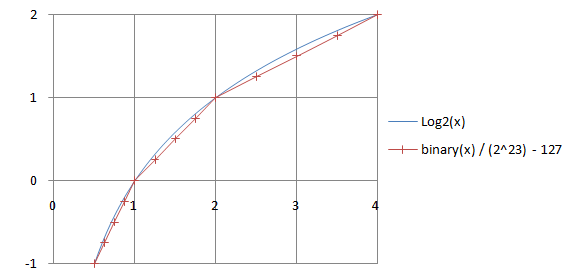
Many computers follow the IEEE (or sufficiently similar) representation, and a very rapid approximation to the square root can be obtained for starting Newton's method. The technique that follows is based on the fact that the floating point format (in base two) approximates the base-2 logarithm. That is

So for a 32-bit single precision floating point number in IEEE format (where notably, the power has a bias of 127 added for the represented form) you can get the approximate logarithm by interpreting its binary representation as a 32-bit integer, scaling it by , and removing a bias of 127, i.e.


For example, 1.0 is represented by a hexadecimal number 0x3F800000, which would represent if taken as an integer. Using the formula above you get , as expected from . In a similar fashion you get 0.5 from 1.5 (0x3FC00000).


To get the square root, divide the logarithm by 2 and convert the value back. The following program demonstrates the idea. Note that the exponent's lowest bit is intentionally allowed to propagate into the mantissa. One way to justify the steps in this program is to assume is the exponent bias and is the number of explicitly stored bits in the mantissa and then show that


/* Assumes that float is in the IEEE 754 single precision floating point format
 * and that int is 32 bits. */
float sqrt_approx(float z) {
    int val_int = *(int*)&z; /* Same bits, but as an int */
    /*
     * To justify the following code, prove that
     *
     * ((((val_int / 2^m) - b) / 2) + b) * 2^m = ((val_int - 2^m) / 2) + ((b + 1) / 2) * 2^m)
     *
     * where
     *
     * b = exponent bias
     * m = number of mantissa bits
     *
     * .
     */

    val_int -= 1 << 23; /* Subtract 2^m. */
    val_int >>= 1; /* Divide by 2. */
    val_int += 1 << 29; /* Add ((b + 1) / 2) * 2^m. */

    return *(float*)&val_int; /* Interpret again as float */
}
The three mathematical operations forming the core of the above function can be expressed in a single line. An additional adjustment can be added to reduce the maximum relative error. So, the three operations, not including the cast, can be rewritten as
val_int = (1 << 29) + (val_int >> 1) - (1 << 22) + a;
where a is a bias for adjusting the approximation errors. For example, with a = 0 the results are accurate for even powers of 2 (e.g., 1.0), but for other numbers the results will be slightly too big (e.g.,1.5 for 2.0 instead of 1.414... with 6% error). With a = -0x4B0D2, the maximum relative error is minimized to ±3.5%.
If the approximation is to be used for an initial guess for Newton's method to the equation , then the reciprocal form shown in the following section is preferred.
Reciprocal of the square root
A variant of the above routine is included below, which can be used to compute the reciprocal of the square root, i.e., instead, was written by Greg Walsh. The integer-shift approximation produced a relative error of less than 4%, and the error dropped further to 0.15% with one iteration of Newton's method on the following line.[10] In computer graphics it is a very efficient way to normalize a vector.

float invSqrt(float x) {
    float xhalf = 0.5f*x;
    union {
        float x;
        int i;
    } u;
    u.x = x;
    u.i = 0x5f375a86 - (u.i >> 1);
    /* The next line can be repeated any number of times to increase accuracy */
    u.x = u.x * (1.5f - xhalf * u.x * u.x);
    return u.x;
}
Some VLSI hardware implements inverse square root using a second degree polynomial estimation followed by a Goldschmidt iteration.[11]
Negative or complex square
If S < 0, then its principal square root is

If S = a+bi where a and b are real and b ≠ 0, then its principal square root is

This can be verified by squaring the root.[12][13] Here

is the modulus of S. The principal square root of a complex number is defined to be the root with the non-negative real part.
Notes
- In addition to the principal square root, there is a negative square root equal in magnitude but opposite in sign to the principal square root, except for zero, which has double square roots of zero.
- The factors two and six are used because they approximate the geometric means of the lowest and highest possible values with the given number of digits: and .
- The unrounded estimate has maximum absolute error of 2.65 at 100 and maximum relative error of 26.5% at y=1, 10 and 100
- If the number is exactly half way between two squares, like 30.5, guess the higher number which is 6 in this case
- This is incidentally the equation of the tangent line to y=x2 at y=1.


References
- Fowler, David; Robson, Eleanor (1998). "Square Root Approximations in Old Babylonian Mathematics: YBC 7289 in Context". Historia Mathematica. 25 (4): 376. doi:10.1006/hmat.1998.2209.
- Heath, Thomas (1921). A History of Greek Mathematics, Vol. 2. Oxford: Clarendon Press. pp. 323–324.
- Bailey, David; Borwein, Jonathan (2012). "Ancient Indian Square Roots: An Exercise in Forensic Paleo-Mathematics" (PDF). American Mathematical Monthly. 119 (8). pp. 646–657. Retrieved 2017-09-14.
- Fast integer square root by Mr. Woo's abacus algorithm (archived)
- Integer Square Root function
- M. V. Wilkes, D. J. Wheeler and S. Gill, "The Preparation of Programs for an Electronic Digital Computer", Addison-Wesley, 1951.
- M. Campbell-Kelly, "Origin of Computing", Scientific American, September 2009.
- J. C. Gower, "A Note on an Iterative Method for Root Extraction", The Computer Journal 1(3):142–143, 1958.
- Markstein, Peter (November 2004). Software Division and Square Root Using Goldschmidt's Algorithms (PDF). 6th Conference on Real Numbers and Computers. Dagstuhl, Germany. CiteSeerX 10.1.1.85.9648.
- Fast Inverse Square Root by Chris Lomont
- "High-Speed Double-Precision Computation of Reciprocal, Division, Square Root and Inverse Square Root" by José-Alejandro Piñeiro and Javier Díaz Bruguera 2002 (abstract)
- Abramowitz, Miltonn; Stegun, Irene A. (1964). Handbook of mathematical functions with formulas, graphs, and mathematical tables. Courier Dover Publications. p. 17. ISBN 978-0-486-61272-0., Section 3.7.26, p. 17
- Cooke, Roger (2008). Classical algebra: its nature, origins, and uses. John Wiley and Sons. p. 59. ISBN 978-0-470-25952-8., Extract: page 59