Harmonic distribution
In probability theory and statistics, the harmonic distribution is a continuous probability distribution. It was discovered by Étienne Halphen, who had become interested in the statistical modeling of natural events. His practical experience in data analysis motivated him to pioneer a new system of distributions that provided sufficient flexibility to fit a large variety of data sets. Halphen restricted his search to distributions whose parameters could be estimated using simple statistical approaches. Then, Halphen introduced for the first time what he called the harmonic distribution or harmonic law. The harmonic law is a special case of the generalized inverse Gaussian distribution family when .

|
Probability density function 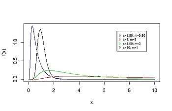 | |||
|
Cumulative distribution function 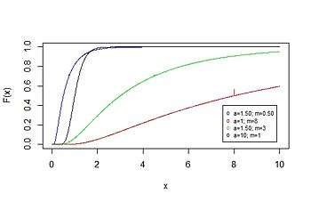 | |||
| Notation | |||
|---|---|---|---|
| Parameters | m ≥ 0, a ≥ 0 | ||
| Support | x > 0 | ||
| Mean | |||
| Median | m | ||
| Mode | |||
| Variance | |||
| Skewness | |||
| Ex. kurtosis | (see text) | ||


History
One of Halphen's tasks, while working as statistician for Electricité de France, was the modeling of the monthly flow of water in hydroelectric stations. Halphen realized that the Pearson system of probability distributions could not be solved; it was inadequate for his purpose despite its remarkable properties. Therefore, Halphen's objective was to obtain a probability distribution with two parameters, subject to an exponential decay both for large and small flows.
In 1941, Halphen decided that, in suitably scaled units, the density of X should be the same as that of 1/X.[1] Taken this consideration, Halphen found the harmonic density function. Nowadays known as a hyperbolic distribution, has been studied by Rukhin (1974) and Barndorff-Nielsen (1978).[2]
The harmonic law is the only one two-parameter family of distributions that is closed under change of scale and under reciprocals, such that the maximum likelihood estimator of the population mean is the sample mean (Gauss' principle).[3]
In 1946, Halphen realized that introducing an additional parameter, flexibility could be improved. His efforts led him to generalize the harmonic law to obtain the generalized inverse Gaussian distribution density.[1]
Definition
Notation
The harmonic distribution will be denoted by . As a result, when a random variable X is distributed following a harmonic law, the parameter of scale m is the population median and a is the parameter of shape.


Probability density function
The density function of the harmonic law, which depends of two parameters,[3] has the form,

where
- denotes the third kind of the modified Bessel function with index 0,


Properties
Moments
To derive an expression for the non-central moment of order r, the integral representation of the Bessel function can be used.[4]

where:
- r denotes the order of the moment.
Hence the mean and the succeeding three moments about it are
| Order | Moment | Cumulant |
|---|---|---|
| 1 | ||
| 2 | ||
| 3 | ||
| 4 |


Skewness
Skewness is the third standardized moment around the mean divided by the 3/2 power of the standard deviation, we work with,[4]

- Always , so the mass of the distribution is concentrated on the left.


Parameter estimation
Maximum likelihood estimation
The likelihood function is

After that, the log-likelihood function is

From the log-likelihood function, the likelihood equations are


These equations admit only a numerical solution for a, but we have

Method of moments
The mean and the variance for the harmonic distribution are,[3][4]

Note that

The method of moments consists in to solve the following equations:

where is the sample variance and is the sample mean. Solving the second equation we obtain , and then we calculate using


Related distributions
The harmonic law is a sub-family of the generalized inverse Gaussian distribution. The density of GIG family have the form

The density of the generalized inverse Gaussian distribution family corresponds to the harmonic law when .[3]
When tends to infinity, the harmonic law can be approximated by a normal distribution. This is indicated by demonstrating that if tends to infinity, then , which is a linear transformation of X, tends to a normal distribution ().


This explains why the normal distribution can be used successfully for certain data sets of ratios.[4]
Another related distribution is the log-harmonic law, which is the probability distribution of a random variable whose logarithm follows an harmonic law.
This family has an interesting property, the Pitman estimator of the location parameter does not depend on the choice of the loss function. Only two statistical models satisfy this property: One is the normal family of distributions and the other one is a three-parameter statistical model which contains the log-harmonic law.[2]
References
- Kots, Samuel L. (1982–1989). Encyclopedia of statistical sciences. 5. pp. 3059–3061 3069–3072.
- Rukhin, A.L. (1978). "Strongly symmetrical families and statistical analysis of their parameters". Journal of Soviet Mathematics. 9: 886–910.
- Puig, Pere (2008). "A note on the harmonic law: A two-parameter family of distributions for ratios". Statistics and Probability Letters. 78: 320–326.
- Perrault, L.; Bobée, B.; Rasmussen, P.F. (1999). "Halphen distribution system. I: Mathematical and statistical properties". J. Hydrol. Eng. 4 (3): 189–199.