Discrete cosine transform
A discrete cosine transform (DCT) expresses a finite sequence of data points in terms of a sum of cosine functions oscillating at different frequencies. The DCT, first proposed by Nasir Ahmed in 1972, is a widely used transformation technique in signal processing and data compression. It is used in most digital media, including digital images (such as JPEG and HEIF, where small high-frequency components can be discarded), digital video (such as MPEG and H.26x), digital audio (such as Dolby Digital, MP3 and AAC), digital television (such as SDTV, HDTV and VOD), digital radio (such as AAC+ and DAB+), and speech coding (such as AAC-LD, Siren and Opus). DCTs are also important to numerous other applications in science and engineering, such as digital signal processing, communications devices, reducing network bandwidth usage, and spectral methods for the numerical solution of partial differential equations.
The use of cosine rather than sine functions is critical for compression, since it turns out (as described below) that fewer cosine functions are needed to approximate a typical signal, whereas for differential equations the cosines express a particular choice of boundary conditions. In particular, a DCT is a Fourier-related transform similar to the discrete Fourier transform (DFT), but using only real numbers. The DCTs are generally related to Fourier Series coefficients of a periodically and symmetrically extended sequence whereas DFTs are related to Fourier Series coefficients of a periodically extended sequence. DCTs are equivalent to DFTs of roughly twice the length, operating on real data with even symmetry (since the Fourier transform of a real and even function is real and even), whereas in some variants the input and/or output data are shifted by half a sample. There are eight standard DCT variants, of which four are common.
The most common variant of discrete cosine transform is the type-II DCT, which is often called simply "the DCT". This was the original DCT as first proposed by Ahmed. Its inverse, the type-III DCT, is correspondingly often called simply "the inverse DCT" or "the IDCT". Two related transforms are the discrete sine transform (DST), which is equivalent to a DFT of real and odd functions, and the modified discrete cosine transform (MDCT), which is based on a DCT of overlapping data. Multidimensional DCTs (MD DCTs) are developed to extend the concept of DCT on MD signals. There are several algorithms to compute MD DCT. A variety of fast algorithms have been developed to reduce the computational complexity of implementing DCT. One of these is the integer DCT[1] (IntDCT), an integer approximation of the standard DCT,[2] used in several ISO/IEC and ITU-T international standards.[2][1]
DCT compression, also known as block compression, compresses data in sets of discrete DCT blocks.[3] DCT blocks can have a number of sizes, including 8x8 pixels for the standard DCT, and varied integer DCT sizes between 4x4 and 32x32 pixels.[1][4] The DCT has a strong "energy compaction" property,[5][6] capable of achieving high quality at high data compression ratios.[7][8] However, blocky compression artifacts can appear when heavy DCT compression is applied.
History
The discrete cosine transform (DCT) was first conceived by Nasir Ahmed, while working at Kansas State University, and he proposed the concept to the National Science Foundation in 1972. He originally intended DCT for image compression.[9][1] Ahmed developed a practical DCT algorithm with his PhD student T. Natarajan and friend K. R. Rao at the University of Texas at Arlington in 1973, and they found that it was the most efficient algorithm for image compression.[9] They presented their results in a January 1974 paper, titled "Discrete Cosine Transform".[5][6][10] It described what is now called the type-II DCT (DCT-II),[11] as well as the type-III inverse DCT (IDCT).[5] It was a benchmark publication,[12][13] and has been cited as a fundamental development in thousands of works since its publication.[14] The basic research work and events that led to the development of the DCT were summarized in a later publication by Ahmed, "How I Came Up with the Discrete Cosine Transform".[9]
Since its introduction in 1974, there has been significant research on the DCT.[10] In 1977, Wen-Hsiung Chen published a paper with C. Harrison Smith and Stanley C. Fralick presenting a fast DCT algorithm,[15][10] and he founded Compression Labs to commercialize DCT technology.[1] Further developments include a 1978 paper by M.J. Narasimha and A.M. Peterson, and a 1984 paper by B.G. Lee.[10] These research papers, along with the original 1974 Ahmed paper and the 1977 Chen paper, were cited by the Joint Photographic Experts Group as the basis for JPEG's lossy image compression algorithm in 1992.[10][16]
In 1975, John A. Roese and Guner S. Robinson adapted the DCT for inter-frame motion-compensated video coding. They experimented with the DCT and the fast Fourier transform (FFT), developing inter-frame hybrid coders for both, and found that the DCT is the most efficient due to its reduced complexity, capable of compressing image data down to 0.25-bit per pixel for a videotelephone scene with image quality comparable to an intra-frame coder requiring 2-bit per pixel.[17][18] The DCT was applied to video encoding by Wen-Hsiung Chen,[1] who developed a fast DCT algorithm with C.H. Smith and S.C. Fralick in 1977,[19][10] and founded Compression Labs to commercialize DCT technology.[1] In 1979, Anil K. Jain and Jaswant R. Jain further developed motion-compensated DCT video compression,[20][21] also called block motion compensation.[21] This led to Chen developing a practical video compression algorithm, called motion-compensated DCT or adaptive scene coding, in 1981.[21] Motion-compensated DCT later became the standard coding technique for video compression from the late 1980s onwards.[22][23]
The integer DCT is used in Advanced Video Coding (AVC),[24][1] introduced in 2003, and High Efficiency Video Coding (HEVC),[4][1] introduced in 2013. The integer DCT is also used in the High Efficiency Image Format (HEIF), which uses a subset of the HEVC video coding format for coding still images.[4]
A DCT variant, the modified discrete cosine transform (MDCT), was developed by John P. Princen, A.W. Johnson and Alan B. Bradley at the University of Surrey in 1987,[25] following earlier work by Princen and Bradley in 1986.[26] The MDCT is used in most modern audio compression formats, such as Dolby Digital (AC-3),[27][28] MP3 (which uses a hybrid DCT-FFT algorithm),[29] Advanced Audio Coding (AAC),[30] and Vorbis (Ogg).[31]
The discrete sine transform (DST) was derived from the DCT, by replacing the Neumann condition at x=0 with a Dirichlet condition.[32] The DST was described in the 1974 DCT paper by Ahmed, Natarajan and Rao.[5] A type-I DST (DST-I) was later described by Anil K. Jain in 1976, and a type-II DST (DST-II) was then described by H.B. Kekra and J.K. Solanka in 1978.[33]
Nasir Ahmed also developed a lossless DCT algorithm with Giridhar Mandyam and Neeraj Magotra at the University of New Mexico in 1995. This allows the DCT technique to be used for lossless compression of images. It is a modification of the original DCT algorithm, and incorporates elements of inverse DCT and delta modulation. It is a more effective lossless compression algorithm than entropy coding.[34] Lossless DCT is also known as LDCT.[35]
Wavelet coding, the use of wavelet transforms in image compression, began after the development of DCT coding.[36] The introduction of the DCT led to the development of wavelet coding, a variant of DCT coding that uses wavelets instead of DCT's block-based algorithm.[36] Discrete wavelet transform (DWT) coding is used in the JPEG 2000 standard,[37] developed from 1997 to 2000.[38] Wavelet coding is more processor-intensive, and it has yet to see widespread deployment in consumer-facing use.[39]
Applications
The DCT is the most widely used transformation technique in signal processing,[40] and by far the most widely used linear transform in data compression.[41] DCT data compression has been fundamental to the Digital Revolution.[8][42][43] Uncompressed digital media as well as lossless compression had impractically high memory and bandwidth requirements, which was significantly reduced by the highly efficient DCT lossy compression technique,[7][8] capable of achieving data compression ratios from 8:1 to 14:1 for near-studio-quality,[7] up to 100:1 for acceptable-quality content.[8] The wide adoption of DCT compression standards led to the emergence and proliferation of digital media technologies, such as digital images, digital photos,[44][45] digital video,[22][43] streaming media,[46] digital television, streaming television, video-on-demand (VOD),[8] digital cinema,[27] high-definition video (HD video), and high-definition television (HDTV).[7][47]
The DCT, and in particular the DCT-II, is often used in signal and image processing, especially for lossy compression, because it has a strong "energy compaction" property:[5][6] in typical applications, most of the signal information tends to be concentrated in a few low-frequency components of the DCT. For strongly correlated Markov processes, the DCT can approach the compaction efficiency of the Karhunen-Loève transform (which is optimal in the decorrelation sense). As explained below, this stems from the boundary conditions implicit in the cosine functions.
DCTs are also widely employed in solving partial differential equations by spectral methods, where the different variants of the DCT correspond to slightly different even/odd boundary conditions at the two ends of the array.
DCTs are also closely related to Chebyshev polynomials, and fast DCT algorithms (below) are used in Chebyshev approximation of arbitrary functions by series of Chebyshev polynomials, for example in Clenshaw–Curtis quadrature.
The DCT is the coding standard for multimedia communications devices. It is widely used for bit rate reduction, and reducing network bandwidth usage.[1] DCT compression significantly reduces the amount of memory and bandwidth required for digital signals.[8]
General applications
The DCT is widely used in many applications, which include the following.
- Audio signal processing — audio coding, audio data compression (lossy and lossless),[48] surround sound,[27] acoustic echo and feedback cancellation, phoneme recognition, time-domain aliasing cancellation (TDAC)[49]
- Digital audio[1]
- Digital radio — Digital Audio Broadcasting (DAB+),[50] HD Radio[51]
- Speech processing — speech coding[52][53] speech recognition, voice activity detection (VAD)[49]
- Digital telephony — voice-over-IP (VoIP),[52] mobile telephony, video telephony,[53] teleconferencing, videoconferencing[1]
- Biometrics — fingerprint orientation, facial recognition systems, biometric watermarking, fingerprint-based biometric watermarking, palm print identification/recognition[49]
- Computers and the Internet — the World Wide Web, social media,[44][45] Internet video[54]
- Network bandwidth usage reducation[1]
- Consumer electronics[49] — multimedia systems,[1] multimedia communications devices,[1] consumer devices[54]
- Cryptography — encryption, steganography, copyright protection[49]
- Data compression — transform coding, lossy compression, lossless compression[48]
- Encoding operations — quantization, perceptual weighting, entropy encoding, variable encoding[1]
- Digital media[46] — digital distribution[55]
- Streaming media[46] — streaming audio, streaming video, streaming television, video-on-demand (VOD)[8]
- Forgery detection[49]
- Geophysical transient electromagnetics (transient EM)[49]
- Images — artist identification,[49] focus and blurriness measure,[49] feature extraction[49]
- Color formatting — formatting luminance and color differences, color formats (such as YUV444 and YUV411), decoding operations such as the inverse operation between display color formats (YIQ, YUV, RGB)[1]
- Digital imaging — digital images, digital cameras, digital photography,[44][45] high-dynamic-range imaging (HDR imaging)[56]
- Image compression[49][57] — image file formats,[58] multiview image compression, progressive image transmission[49]
- Image processing — digital image processing,[1] image analysis, content-based image retrieval, corner detection, directional block-wise image representation, edge detection, image enhancement, image fusion, image segmentation, interpolation, image noise level estimation, mirroring, rotation, just-noticeable distortion (JND) profile, spatiotemporal masking effects, foveated imaging[49]
- Image quality assessment — DCT-based quality degradation metric (DCT QM)[49]
- Image reconstruction — directional textures auto inspection, image restoration, inpainting, visual recovery[49]
- Medical technology
- Electrocardiography (ECG) — vectorcardiography (VCG)[49]
- Medical imaging — medical image compression, image fusion, watermarking, brain tumor compression classification[49]
- Pattern recognition[49]
- Region of interest (ROI) extraction[49]
- Signal processing — digital signal processing, digital signal processors (DSP), DSP software, multiplexing, signaling, control signals, analog-to-digital conversion (ADC),[1] compressive sampling, DCT pyramid error concealment, downsampling, upsampling, signal-to-noise ratio (SNR) estimation, transmux, Wiener filter[49]
- Surveillance[49]
- Vehicular black box camera[49]
- Video
- Digital cinema[57] — digital cinematography, digital movie cameras, video editing, film editing,[59][60] Dolby Digital audio[1][27]
- Digital television (DTV)[7] — digital television broadcasting,[57] standard-definition television (SDTV), high-definition TV (HDTV),[7][47] HDTV encoder/decoder chips, ultra HDTV (UHDTV)[1]
- Digital video[22][43] — digital versatile disc (DVD),[57] high-definition (HD) video[7][47]
- Video coding — video compression,[1] video coding standards,[49] motion estimation, motion compensation, inter-frame prediction, motion vectors,[1] 3D video coding, local distortion detection probability (LDDP) model, moving object detection, Multiview Video Coding (MVC)[49]
- Video processing — motion analysis, 3D-DCT motion analysis, video content analysis, data extraction,[49] video browsing,[61] professional video production[62]
- Watermarking — digital watermarking, image watermarking, video watermarking, 3D video watermarking, reversible data hiding, watermarking detection[49]
- Wireless technology
- Mobile devices[54] — mobile phones, smartphones,[53] videophones[1]
- Radio frequency (RF) technology — RF engineering, aperture arrays,[49] beamforming, digital arithmetic circuits, directional sensing, space imaging[63]
- Wireless sensor network (WSN) — wireless acoustic sensor networks[49]
DCT visual media standards
The DCT-II, also known as simply the DCT, is the most important image compression technique. It is used in image compression standards such as JPEG, and video compression standards such as H.26x, MJPEG, MPEG, DV, Theora and Daala. There, the two-dimensional DCT-II of blocks are computed and the results are quantized and entropy coded. In this case, is typically 8 and the DCT-II formula is applied to each row and column of the block. The result is an 8 × 8 transform coefficient array in which the element (top-left) is the DC (zero-frequency) component and entries with increasing vertical and horizontal index values represent higher vertical and horizontal spatial frequencies.


Advanced Video Coding (AVC) uses the integer DCT[24][1] (IntDCT), an integer approximation of the DCT.[2][1] It uses 4x4 and 8x8 integer DCT blocks. High Efficiency Video Coding (HEVC) and the High Efficiency Image Format (HEIC) use varied integer DCT block sizes between 4x4 and 32x32 pixels.[4][1] As of 2019, AVC is by far the most commonly used format for the recording, compression and distribution of video content, used by 91% of video developers, followed by HEVC which is used by 43% of developers.[55]
Image formats
| Image compression standard | Year | Common applications |
|---|---|---|
| JPEG[1] | 1992 | The most widely used image compression standard[64][65] and digital image format,[58] |
| JPEG XR | 2009 | Open XML Paper Specification |
| WebP | 2010 | A graphic format that supports the lossy compression of digital images. Developed by Google. |
| High Efficiency Image Format (HEIF) | 2013 | Image file format based on HEVC compression. It improves compression over JPEG,[66] and supports animation with much more efficient compression than the animated GIF format.[67] |
| BPG | 2014 | Based on HEVC compression |
Video formats
| Video coding standard | Year | Common applications |
|---|---|---|
| H.261[68][69] | 1988 | First of a family of video coding standards. Used primarily in older video conferencing and video telephone products. |
| Motion JPEG (MJPEG)[70] | 1992 | QuickTime, video editing, non-linear editing, digital cameras |
| MPEG-1 Video[71] | 1993 | Digital video distribution on CD or via the World Wide Web. |
| MPEG-2 Video (H.262)[71] | 1995 | Storage and handling of digital images in broadcast applications, digital television, HDTV, cable, satellite, high-speed Internet, DVD video distribution |
| DV | 1995 | Camcorders, digital cassettes |
| H.263 (MPEG-4 Part 2)[68] | 1996 | Video telephony over public switched telephone network (PSTN), H.320, Integrated Services Digital Network (ISDN)[72][73] |
| Advanced Video Coding (AVC / H.264 / MPEG-4)[1][24] | 2003 | Most common HD video recording/compression/distribution format, streaming Internet video, YouTube, Blu-ray Discs, HDTV broadcasts, web browsers, streaming television, mobile devices, consumer devices, Netflix,[54] video telephony, Facetime[53] |
| Theora | 2004 | Internet video, web browsers |
| VC-1 | 2006 | Windows media, Blu-ray Discs |
| Apple ProRes | 2007 | Professional video production.[62] |
| WebM Video | 2010 | A multimedia open source format developed by Google intended to be used with HTML5. |
| High Efficiency Video Coding (HEVC / H.265)[1][4] | 2013 | The emerging successor to the H.264/MPEG-4 AVC standard, having substantially improved compression capability. |
| Daala | 2013 |
MDCT audio standards
General audio
Speech coding
| Speech coding standard | Year | Common applications |
|---|---|---|
| AAC-LD (LD-MDCT)[78] | 1999 | Mobile telephony, voice-over-IP (VoIP), iOS, FaceTime[53] |
| Siren[52] | 1999 | VoIP, wideband audio, G.722.1 |
| G.722.1[79] | 1999 | VoIP, wideband audio, G.722 |
| G.729.1[80] | 2006 | G.729, VoIP, wideband audio,[80] mobile telephony |
| EVRC-WB[81] | 2007 | Wideband audio |
| G.718[82] | 2008 | VoIP, wideband audio, mobile telephony |
| G.719[81] | 2008 | Teleconferencing, videoconferencing, voice mail |
| CELT[83] | 2011 | VoIP,[84][85] mobile telephony |
| Opus[86] | 2012 | VoIP,[87] mobile telephony, WhatsApp,[88][89][90] PlayStation 4[91] |
| Enhanced Voice Services (EVS)[92] | 2014 | Mobile telephony, VoIP, wideband audio |
MD DCT
Multidimensional DCTs (MD DCTs) have several applications, mainly 3-D DCTs such as the 3-D DCT-II, which has several new applications like Hyperspectral Imaging coding systems,[93] variable temporal length 3-D DCT coding,[94] video coding algorithms,[95] adaptive video coding [96] and 3-D Compression.[97] Due to enhancement in the hardware, software and introduction of several fast algorithms, the necessity of using M-D DCTs is rapidly increasing. DCT-IV has gained popularity for its applications in fast implementation of real-valued polyphase filtering banks,[98] lapped orthogonal transform[99][100] and cosine-modulated wavelet bases.[101]
Digital signal processing
DCT plays a very important role in digital signal processing. By using the DCT, the signals can be compressed. DCT can be used in electrocardiography for the compression of ECG signals. DCT2 provides a better compression ratio than DCT.
The DCT is widely implemented in digital signal processors (DSP), as well as digital signal processing software. Many companies have developed DSPs based on DCT technology. DCTs are widely used for applications such as encoding, decoding, video, audio, multiplexing, control signals, signaling, and analog-to-digital conversion. DCTs are also commonly used for high-definition television (HDTV) encoder/decoder chips.[1]
Compression artifacts
A common issue with DCT compression in digital media are blocky compression artifacts,[102] caused by DCT blocks.[3] The DCT algorithm can cause block-based artifacts when heavy compression is applied. Due to the DCT being used in the majority of digital image and video coding standards (such as the JPEG, H.26x and MPEG formats), DCT-based blocky compression artifacts are widespread in digital media. In a DCT algorithm, an image (or frame in an image sequence) is divided into square blocks which are processed independently from each other, then the DCT of these blocks is taken, and the resulting DCT coefficients are quantized. This process can cause blocking artifacts, primarily at high data compression ratios.[102] This can also cause the "mosquito noise" effect, commonly found in digital video (such as the MPEG formats).[103]
DCT blocks are often used in glitch art.[3] The artist Rosa Menkman makes use of DCT-based compression artifacts in her glitch art,[104] particularly the DCT blocks found in most digital media formats such as JPEG digital images and MP3 digital audio.[3] Another example is Jpegs by German photographer Thomas Ruff, which uses intentional JPEG artifacts as the basis of the picture's style.[105][106]
Informal overview
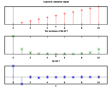
Like any Fourier-related transform, discrete cosine transforms (DCTs) express a function or a signal in terms of a sum of sinusoids with different frequencies and amplitudes. Like the discrete Fourier transform (DFT), a DCT operates on a function at a finite number of discrete data points. The obvious distinction between a DCT and a DFT is that the former uses only cosine functions, while the latter uses both cosines and sines (in the form of complex exponentials). However, this visible difference is merely a consequence of a deeper distinction: a DCT implies different boundary conditions from the DFT or other related transforms.
The Fourier-related transforms that operate on a function over a finite domain, such as the DFT or DCT or a Fourier series, can be thought of as implicitly defining an extension of that function outside the domain. That is, once you write a function as a sum of sinusoids, you can evaluate that sum at any , even for where the original was not specified. The DFT, like the Fourier series, implies a periodic extension of the original function. A DCT, like a cosine transform, implies an even extension of the original function.


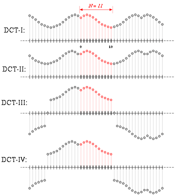
However, because DCTs operate on finite, discrete sequences, two issues arise that do not apply for the continuous cosine transform. First, one has to specify whether the function is even or odd at both the left and right boundaries of the domain (i.e. the min-n and max-n boundaries in the definitions below, respectively). Second, one has to specify around what point the function is even or odd. In particular, consider a sequence abcd of four equally spaced data points, and say that we specify an even left boundary. There are two sensible possibilities: either the data are even about the sample a, in which case the even extension is dcbabcd, or the data are even about the point halfway between a and the previous point, in which case the even extension is dcbaabcd (a is repeated).
These choices lead to all the standard variations of DCTs and also discrete sine transforms (DSTs). Each boundary can be either even or odd (2 choices per boundary) and can be symmetric about a data point or the point halfway between two data points (2 choices per boundary), for a total of 2 × 2 × 2 × 2 = 16 possibilities. Half of these possibilities, those where the left boundary is even, correspond to the 8 types of DCT; the other half are the 8 types of DST.
These different boundary conditions strongly affect the applications of the transform and lead to uniquely useful properties for the various DCT types. Most directly, when using Fourier-related transforms to solve partial differential equations by spectral methods, the boundary conditions are directly specified as a part of the problem being solved. Or, for the MDCT (based on the type-IV DCT), the boundary conditions are intimately involved in the MDCT's critical property of time-domain aliasing cancellation. In a more subtle fashion, the boundary conditions are responsible for the "energy compactification" properties that make DCTs useful for image and audio compression, because the boundaries affect the rate of convergence of any Fourier-like series.
In particular, it is well known that any discontinuities in a function reduce the rate of convergence of the Fourier series, so that more sinusoids are needed to represent the function with a given accuracy. The same principle governs the usefulness of the DFT and other transforms for signal compression; the smoother a function is, the fewer terms in its DFT or DCT are required to represent it accurately, and the more it can be compressed. (Here, we think of the DFT or DCT as approximations for the Fourier series or cosine series of a function, respectively, in order to talk about its "smoothness".) However, the implicit periodicity of the DFT means that discontinuities usually occur at the boundaries: any random segment of a signal is unlikely to have the same value at both the left and right boundaries. (A similar problem arises for the DST, in which the odd left boundary condition implies a discontinuity for any function that does not happen to be zero at that boundary.) In contrast, a DCT where both boundaries are even always yields a continuous extension at the boundaries (although the slope is generally discontinuous). This is why DCTs, and in particular DCTs of types I, II, V, and VI (the types that have two even boundaries) generally perform better for signal compression than DFTs and DSTs. In practice, a type-II DCT is usually preferred for such applications, in part for reasons of computational convenience.
Formal definition
Formally, the discrete cosine transform is a linear, invertible function (where denotes the set of real numbers), or equivalently an invertible N × N square matrix. There are several variants of the DCT with slightly modified definitions. The N real numbers x0, ..., xN-1 are transformed into the N real numbers X0, ..., XN-1 according to one of the formulas:


DCT-I

Some authors further multiply the x0 and xN-1 terms by √2, and correspondingly multiply the X0 and XN-1 terms by 1/√2. This makes the DCT-I matrix orthogonal, if one further multiplies by an overall scale factor of , but breaks the direct correspondence with a real-even DFT.

The DCT-I is exactly equivalent (up to an overall scale factor of 2), to a DFT of real numbers with even symmetry. For example, a DCT-I of N=5 real numbers abcde is exactly equivalent to a DFT of eight real numbers abcdedcb (even symmetry), divided by two. (In contrast, DCT types II-IV involve a half-sample shift in the equivalent DFT.)

Note, however, that the DCT-I is not defined for N less than 2. (All other DCT types are defined for any positive N.)
Thus, the DCT-I corresponds to the boundary conditions: xn is even around n = 0 and even around n = N−1; similarly for Xk.
DCT-II

The DCT-II is probably the most commonly used form, and is often simply referred to as "the DCT".[5][6]
This transform is exactly equivalent (up to an overall scale factor of 2) to a DFT of real inputs of even symmetry where the even-indexed elements are zero. That is, it is half of the DFT of the inputs , where , for , , and for . DCT II transformation is also possible using 2N signal followed by a multiplication by half shift. This is demonstrated by Makhoul.


Some authors further multiply the X0 term by 1/√2 and multiply the resulting matrix by an overall scale factor of (see below for the corresponding change in DCT-III). This makes the DCT-II matrix orthogonal, but breaks the direct correspondence with a real-even DFT of half-shifted input. This is the normalization used by Matlab, for example.[107] In many applications, such as JPEG, the scaling is arbitrary because scale factors can be combined with a subsequent computational step (e.g. the quantization step in JPEG[108]), and a scaling can be chosen that allows the DCT to be computed with fewer multiplications.[109][110]

The DCT-II implies the boundary conditions: xn is even around n = −1/2 and even around n = N−1/2; Xk is even around k = 0 and odd around k = N.
DCT-III

Because it is the inverse of DCT-II (up to a scale factor, see below), this form is sometimes simply referred to as "the inverse DCT" ("IDCT").[6]
Some authors divide the x0 term by √2 instead of by 2 (resulting in an overall x0/√2 term) and multiply the resulting matrix by an overall scale factor of (see above for the corresponding change in DCT-II), so that the DCT-II and DCT-III are transposes of one another. This makes the DCT-III matrix orthogonal, but breaks the direct correspondence with a real-even DFT of half-shifted output.
The DCT-III implies the boundary conditions: xn is even around n = 0 and odd around n = N; Xk is even around k = −1/2 and even around k = N−1/2.
DCT-IV

The DCT-IV matrix becomes orthogonal (and thus, being clearly symmetric, its own inverse) if one further multiplies by an overall scale factor of .

A variant of the DCT-IV, where data from different transforms are overlapped, is called the modified discrete cosine transform (MDCT).[111]
The DCT-IV implies the boundary conditions: xn is even around n = −1/2 and odd around n = N−1/2; similarly for Xk.
DCT V-VIII
DCTs of types I-IV treat both boundaries consistently regarding the point of symmetry: they are even/odd around either a data point for both boundaries or halfway between two data points for both boundaries. By contrast, DCTs of types V-VIII imply boundaries that are even/odd around a data point for one boundary and halfway between two data points for the other boundary.
In other words, DCT types I-IV are equivalent to real-even DFTs of even order (regardless of whether N is even or odd), since the corresponding DFT is of length 2(N−1) (for DCT-I) or 4N (for DCT-II/III) or 8N (for DCT-IV). The four additional types of discrete cosine transform[112] correspond essentially to real-even DFTs of logically odd order, which have factors of N ± ½ in the denominators of the cosine arguments.
However, these variants seem to be rarely used in practice. One reason, perhaps, is that FFT algorithms for odd-length DFTs are generally more complicated than FFT algorithms for even-length DFTs (e.g. the simplest radix-2 algorithms are only for even lengths), and this increased intricacy carries over to the DCTs as described below.
(The trivial real-even array, a length-one DFT (odd length) of a single number a, corresponds to a DCT-V of length N = 1.)
Inverse transforms
Using the normalization conventions above, the inverse of DCT-I is DCT-I multiplied by 2/(N-1). The inverse of DCT-IV is DCT-IV multiplied by 2/N. The inverse of DCT-II is DCT-III multiplied by 2/N and vice versa.[6]
Like for the DFT, the normalization factor in front of these transform definitions is merely a convention and differs between treatments. For example, some authors multiply the transforms by so that the inverse does not require any additional multiplicative factor. Combined with appropriate factors of √2 (see above), this can be used to make the transform matrix orthogonal.
Multidimensional DCTs
Multidimensional variants of the various DCT types follow straightforwardly from the one-dimensional definitions: they are simply a separable product (equivalently, a composition) of DCTs along each dimension.
M-D DCT-II
For example, a two-dimensional DCT-II of an image or a matrix is simply the one-dimensional DCT-II, from above, performed along the rows and then along the columns (or vice versa). That is, the 2D DCT-II is given by the formula (omitting normalization and other scale factors, as above):
- The inverse of a multi-dimensional DCT is just a separable product of the inverse(s) of the corresponding one-dimensional DCT(s) (see above), e.g. the one-dimensional inverses applied along one dimension at a time in a row-column algorithm.

The 3-D DCT-II is only the extension of 2-D DCT-II in three dimensional space and mathematically can be calculated by the formula

The inverse of 3-D DCT-II is 3-D DCT-III and can be computed from the formula given by

Technically, computing a two-, three- (or -multi) dimensional DCT by sequences of one-dimensional DCTs along each dimension is known as a row-column algorithm. As with multidimensional FFT algorithms, however, there exist other methods to compute the same thing while performing the computations in a different order (i.e. interleaving/combining the algorithms for the different dimensions). Owing to the rapid growth in the applications based on the 3-D DCT, several fast algorithms are developed for the computation of 3-D DCT-II. Vector-Radix algorithms are applied for computing M-D DCT to reduce the computational complexity and to increase the computational speed. To compute 3-D DCT-II efficiently, a fast algorithm, Vector-Radix Decimation in Frequency (VR DIF) algorithm was developed.
3-D DCT-II VR DIF
In order to apply the VR DIF algorithm the input data is to be formulated and rearranged as follows.[113][114] The transform size N x N x N is assumed to be 2.
- where


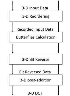
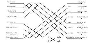
The figure to the adjacent shows the four stages that are involved in calculating 3-D DCT-II using VR DIF algorithm. The first stage is the 3-D reordering using the index mapping illustrated by the above equations. The second stage is the butterfly calculation. Each butterfly calculates eight points together as shown in the figure just below, where .

The original 3-D DCT-II now can be written as

where .

If the even and the odd parts of and and are considered, the general formula for the calculation of the 3-D DCT-II can be expressed as


where


Arithmetic complexity
The whole 3-D DCT calculation needs stages, and each stage involves butterflies. The whole 3-D DCT requires butterflies to be computed. Each butterfly requires seven real multiplications (including trivial multiplications) and 24 real additions (including trivial additions). Therefore, the total number of real multiplications needed for this stage is , and the total number of real additions i.e. including the post-additions (recursive additions) which can be calculated directly after the butterfly stage or after the bit-reverse stage are given by[114] .


The conventional method to calculate MD-DCT-II is using a Row-Column-Frame (RCF) approach which is computationally complex and less productive on most advanced recent hardware platforms. The number of multiplications required to compute VR DIF Algorithm when compared to RCF algorithm are quite a few in number. The number of Multiplications and additions involved in RCF approach are given by and respectively. From Table 1, it can be seen that the total number


| Transform Size | 3D VR Mults | RCF Mults | 3D VR Adds | RCF Adds |
|---|---|---|---|---|
| 8 x 8 x 8 | 2.625 | 4.5 | 10.875 | 10.875 |
| 16 x 16 x 16 | 3.5 | 6 | 15.188 | 15.188 |
| 32 x 32 x 32 | 4.375 | 7.5 | 19.594 | 19.594 |
| 64 x 64 x 64 | 5.25 | 9 | 24.047 | 24.047 |
of multiplications associated with the 3-D DCT VR algorithm is less than that associated with the RCF approach by more than 40%. In addition, the RCF approach involves matrix transpose and more indexing and data swapping than the new VR algorithm. This makes the 3-D DCT VR algorithm more efficient and better suited for 3-D applications that involve the 3-D DCT-II such as video compression and other 3-D image processing applications. The main consideration in choosing a fast algorithm is to avoid computational and structural complexities. As the technology of computers and DSPs advances, the execution time of arithmetic operations (multiplications and additions) is becoming very fast, and regular computational structure becomes the most important factor.[115] Therefore, although the above proposed 3-D VR algorithm does not achieve the theoretical lower bound on the number of multiplications,[116] it has a simpler computational structure as compared to other 3-D DCT algorithms. It can be implemented in place using a single butterfly and possesses the properties of the Cooley–Tukey FFT algorithm in 3-D. Hence, the 3-D VR presents a good choice for reducing arithmetic operations in the calculation of the 3-D DCT-II while keeping the simple structure that characterize butterfly style Cooley–Tukey FFT algorithms.
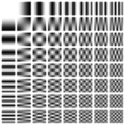
The image to the right shows a combination of horizontal and vertical frequencies for an 8 x 8 () two-dimensional DCT. Each step from left to right and top to bottom is an increase in frequency by 1/2 cycle.

For example, moving right one from the top-left square yields a half-cycle increase in the horizontal frequency. Another move to the right yields two half-cycles. A move down yields two half-cycles horizontally and a half-cycle vertically. The source data (8x8) is transformed to a linear combination of these 64 frequency squares.
MD-DCT-IV
The M-D DCT-IV is just an extension of 1-D DCT-IV on to M dimensional domain. The 2-D DCT-IV of a matrix or an image is given by
- .

We can compute the MD DCT-IV using the regular row-column method or we can use the polynomial transform method[117] for the fast and efficient computation. The main idea of this algorithm is to use the Polynomial Transform to convert the multidimensional DCT into a series of 1-D DCTs directly. MD DCT-IV also has several applications in various fields.
Computation
Although the direct application of these formulas would require O(N2) operations, it is possible to compute the same thing with only O(N log N) complexity by factorizing the computation similarly to the fast Fourier transform (FFT). One can also compute DCTs via FFTs combined with O(N) pre- and post-processing steps. In general, O(N log N) methods to compute DCTs are known as fast cosine transform (FCT) algorithms.
The most efficient algorithms, in principle, are usually those that are specialized directly for the DCT, as opposed to using an ordinary FFT plus O(N) extra operations (see below for an exception). However, even "specialized" DCT algorithms (including all of those that achieve the lowest known arithmetic counts, at least for power-of-two sizes) are typically closely related to FFT algorithms—since DCTs are essentially DFTs of real-even data, one can design a fast DCT algorithm by taking an FFT and eliminating the redundant operations due to this symmetry. This can even be done automatically (Frigo & Johnson, 2005). Algorithms based on the Cooley–Tukey FFT algorithm are most common, but any other FFT algorithm is also applicable. For example, the Winograd FFT algorithm leads to minimal-multiplication algorithms for the DFT, albeit generally at the cost of more additions, and a similar algorithm was proposed by Feig & Winograd (1992) for the DCT. Because the algorithms for DFTs, DCTs, and similar transforms are all so closely related, any improvement in algorithms for one transform will theoretically lead to immediate gains for the other transforms as well (Duhamel & Vetterli 1990).
While DCT algorithms that employ an unmodified FFT often have some theoretical overhead compared to the best specialized DCT algorithms, the former also have a distinct advantage: highly optimized FFT programs are widely available. Thus, in practice, it is often easier to obtain high performance for general lengths N with FFT-based algorithms. (Performance on modern hardware is typically not dominated simply by arithmetic counts, and optimization requires substantial engineering effort.) Specialized DCT algorithms, on the other hand, see widespread use for transforms of small, fixed sizes such as the DCT-II used in JPEG compression, or the small DCTs (or MDCTs) typically used in audio compression. (Reduced code size may also be a reason to use a specialized DCT for embedded-device applications.)

In fact, even the DCT algorithms using an ordinary FFT are sometimes equivalent to pruning the redundant operations from a larger FFT of real-symmetric data, and they can even be optimal from the perspective of arithmetic counts. For example, a type-II DCT is equivalent to a DFT of size with real-even symmetry whose even-indexed elements are zero. One of the most common methods for computing this via an FFT (e.g. the method used in FFTPACK and FFTW) was described by Narasimha & Peterson (1978) and Makhoul (1980), and this method in hindsight can be seen as one step of a radix-4 decimation-in-time Cooley–Tukey algorithm applied to the "logical" real-even DFT corresponding to the DCT II. (The radix-4 step reduces the size DFT to four size- DFTs of real data, two of which are zero and two of which are equal to one another by the even symmetry, hence giving a single size- FFT of real data plus butterflies.) Because the even-indexed elements are zero, this radix-4 step is exactly the same as a split-radix step; if the subsequent size- real-data FFT is also performed by a real-data split-radix algorithm (as in Sorensen et al. 1987), then the resulting algorithm actually matches what was long the lowest published arithmetic count for the power-of-two DCT-II ( real-arithmetic operations[lower-alpha 1]). A recent reduction in the operation count to also uses a real-data FFT.[118] So, there is nothing intrinsically bad about computing the DCT via an FFT from an arithmetic perspective—it is sometimes merely a question of whether the corresponding FFT algorithm is optimal. (As a practical matter, the function-call overhead in invoking a separate FFT routine might be significant for small , but this is an implementation rather than an algorithmic question since it can be solved by unrolling/inlining.)


Example of IDCT
Consider this 8x8 grayscale image of capital letter A.

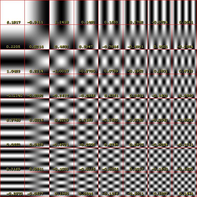
DCT of the image = .

Each basis function is multiplied by its coefficient and then this product is added to the final image.

See also
- Discrete wavelet transform
- JPEG#Discrete cosine transform — Contains a potentially easier to understand example of DCT transformation
- List of Fourier-related transforms
- Modified discrete cosine transform
Explanatory notes
- The precise count of real arithmetic operations, and in particular the count of real multiplications, depends somewhat on the scaling of the transform definition. The count is for the DCT-II definition shown here; two multiplications can be saved if the transform is scaled by an overall factor. Additional multiplications can be saved if one permits the outputs of the transform to be rescaled individually, as was shown by Arai, Agui & Nakajima (1988) for the size-8 case used in JPEG.

Citations
- Stanković, Radomir S.; Astola, Jaakko T. (2012). "Reminiscences of the Early Work in DCT: Interview with K.R. Rao" (PDF). Reprints from the Early Days of Information Sciences. 60. Retrieved 13 October 2019.
- Britanak, Vladimir; Yip, Patrick C.; Rao, K. R. (2010). Discrete Cosine and Sine Transforms: General Properties, Fast Algorithms and Integer Approximations. Elsevier. pp. ix, xiii, 1, 141–304. ISBN 9780080464640.
- Alikhani, Darya (April 1, 2015). "Beyond resolution: Rosa Menkman's glitch art". POSTmatter. Retrieved 19 October 2019.
- Thomson, Gavin; Shah, Athar (2017). "Introducing HEIF and HEVC" (PDF). Apple Inc. Retrieved 5 August 2019.
- Ahmed, Nasir; Natarajan, T.; Rao, K. R. (January 1974), "Discrete Cosine Transform" (PDF), IEEE Transactions on Computers, C-23 (1): 90–93, doi:10.1109/T-C.1974.223784
- Rao, K. R.; Yip, P. (1990), Discrete Cosine Transform: Algorithms, Advantages, Applications, Boston: Academic Press, ISBN 978-0-12-580203-1
- Barbero, M.; Hofmann, H.; Wells, N. D. (14 November 1991). "DCT source coding and current implementations for HDTV". EBU Technical Review. European Broadcasting Union (251): 22–33. Retrieved 4 November 2019.
- Lea, William (1994). "Video on demand: Research Paper 94/68". House of Commons Library. 9 May 1994. Retrieved 20 September 2019.CS1 maint: location (link)
- Ahmed, Nasir (January 1991). "How I Came Up With the Discrete Cosine Transform". Digital Signal Processing. 1 (1): 4–5. doi:10.1016/1051-2004(91)90086-Z.
- "T.81 – Digital compression and coding of continuous-tone still images – Requirements and guidelines" (PDF). CCITT. September 1992. Retrieved 12 July 2019.
- Britanak, Vladimir; Yip, Patrick C.; Rao, K. R. (2010). Discrete Cosine and Sine Transforms: General Properties, Fast Algorithms and Integer Approximations. Elsevier. p. 51. ISBN 9780080464640.
- Selected Papers on Visual Communication: Technology and Applications, (SPIE Press Book), Editors T. Russell Hsing and Andrew G. Tescher, April 1990, pp. 145-149 .
- Selected Papers and Tutorial in Digital Image Processing and Analysis, Volume 1, Digital Image Processing and Analysis, (IEEE Computer Society Press), Editors R. Chellappa and A. A. Sawchuk, June 1985, p. 47.
- DCT citations via Google Scholar .
- Chen, Wen-Hsiung; Smith, C. H.; Fralick, S. C. (September 1977). "A Fast Computational Algorithm for the Discrete Cosine Transform". IEEE Transactions on Communications. 25 (9): 1004–1009. doi:10.1109/TCOM.1977.1093941.
- Smith, C.; Fralick, S. (1977). "A Fast Computational Algorithm for the Discrete Cosine Transform". IEEE Transactions on Communications. 25 (9): 1004–1009. doi:10.1109/TCOM.1977.1093941. ISSN 0090-6778.
- Huang, T. S. (1981). Image Sequence Analysis. Springer Science & Business Media. p. 29. ISBN 9783642870378.
- Roese, John A.; Robinson, Guner S. (30 October 1975). "Combined Spatial And Temporal Coding Of Digital Image Sequences". Efficient Transmission of Pictorial Information. International Society for Optics and Photonics. 0066: 172–181. Bibcode:1975SPIE...66..172R. doi:10.1117/12.965361.
- Chen, Wen-Hsiung; Smith, C. H.; Fralick, S. C. (September 1977). "A Fast Computational Algorithm for the Discrete Cosine Transform". IEEE Transactions on Communications. 25 (9): 1004–1009. doi:10.1109/TCOM.1977.1093941.
- Cianci, Philip J. (2014). High Definition Television: The Creation, Development and Implementation of HDTV Technology. McFarland. p. 63. ISBN 9780786487974.
- "History of Video Compression". ITU-T. Joint Video Team (JVT) of ISO/IEC MPEG & ITU-T VCEG (ISO/IEC JTC1/SC29/WG11 and ITU-T SG16 Q.6). July 2002. pp. 11, 24–9, 33, 40–1, 53–6. Retrieved 3 November 2019.
- Ghanbari, Mohammed (2003). Standard Codecs: Image Compression to Advanced Video Coding. Institution of Engineering and Technology. pp. 1–2. ISBN 9780852967102.
- Li, Jian Ping (2006). Proceedings of the International Computer Conference 2006 on Wavelet Active Media Technology and Information Processing: Chongqing, China, 29-31 August 2006. World Scientific. p. 847. ISBN 9789812709998.
- Wang, Hanli; Kwong, S.; Kok, C. (2006). "Efficient prediction algorithm of integer DCT coefficients for H.264/AVC optimization". IEEE Transactions on Circuits and Systems for Video Technology. 16 (4): 547–552. doi:10.1109/TCSVT.2006.871390.
- Princen, John P.; Johnson, A.W.; Bradley, Alan B. (1987). "Subband/Transform coding using filter bank designs based on time domain aliasing cancellation". ICASSP '87. IEEE International Conference on Acoustics, Speech, and Signal Processing. 12: 2161–2164. doi:10.1109/ICASSP.1987.1169405.
- John P. Princen, Alan B. Bradley: Analysis/synthesis filter bank design based on time domain aliasing cancellation, IEEE Trans. Acoust. Speech Signal Processing, ASSP-34 (5), 1153–1161, 1986
- Luo, Fa-Long (2008). Mobile Multimedia Broadcasting Standards: Technology and Practice. Springer Science & Business Media. p. 590. ISBN 9780387782638.
- Britanak, V. (2011). "On Properties, Relations, and Simplified Implementation of Filter Banks in the Dolby Digital (Plus) AC-3 Audio Coding Standards". IEEE Transactions on Audio, Speech, and Language Processing. 19 (5): 1231–1241. doi:10.1109/TASL.2010.2087755.
- Guckert, John (Spring 2012). "The Use of FFT and MDCT in MP3 Audio Compression" (PDF). University of Utah. Retrieved 14 July 2019.
- Brandenburg, Karlheinz (1999). "MP3 and AAC Explained" (PDF). Archived (PDF) from the original on 2017-02-13.
- Xiph.Org Foundation (2009-06-02). "Vorbis I specification - 1.1.2 Classification". Xiph.Org Foundation. Retrieved 2009-09-22.
- Britanak, Vladimir; Yip, Patrick C.; Rao, K. R. (2010). Discrete Cosine and Sine Transforms: General Properties, Fast Algorithms and Integer Approximations. Elsevier. pp. 35–6. ISBN 9780080464640.
- Dhamija, Swati; Jain, Priyanka (September 2011). "Comparative Analysis for Discrete Sine Transform as a suitable method for noise estimation". IJCSI International Journal of Computer Science. 8 (Issue 5, No. 3): 162-164 (162). Retrieved 4 November 2019.
- Mandyam, Giridhar D.; Ahmed, Nasir; Magotra, Neeraj (17 April 1995). "DCT-based scheme for lossless image compression". Digital Video Compression: Algorithms and Technologies 1995. International Society for Optics and Photonics. 2419: 474–478. Bibcode:1995SPIE.2419..474M. doi:10.1117/12.206386. S2CID 13894279.
- Komatsu, K.; Sezaki, Kaoru (1998). "Reversible discrete cosine transform". Proceedings of the 1998 IEEE International Conference on Acoustics, Speech and Signal Processing, ICASSP '98 (Cat. No.98CH36181). 3: 1769–1772 vol.3. doi:10.1109/ICASSP.1998.681802. ISBN 0-7803-4428-6.
- Hoffman, Roy (2012). Data Compression in Digital Systems. Springer Science & Business Media. p. 124. ISBN 9781461560319.
Basically, wavelet coding is a variant on DCT-based transform coding that reduces or eliminates some of its limitations. (...) Another advantage is that rather than working with 8 × 8 blocks of pixels, as do JPEG and other block-based DCT techniques, wavelet coding can simultaneously compress the entire image.
- Unser, M.; Blu, T. (2003). "Mathematical properties of the JPEG2000 wavelet filters". IEEE Transactions on Image Processing. 12 (9): 1080–1090. Bibcode:2003ITIP...12.1080U. doi:10.1109/TIP.2003.812329. PMID 18237979. S2CID 2765169.
- Taubman, David; Marcellin, Michael (2012). JPEG2000 Image Compression Fundamentals, Standards and Practice: Image Compression Fundamentals, Standards and Practice. Springer Science & Business Media. ISBN 9781461507994.
- McKernan, Brian (2005). Digital cinema: the revolution in cinematography, postproduction, and distribution. McGraw-Hill. p. 59. ISBN 978-0-07-142963-4.
Wavelets have been used in a number of systems, but the technology is more processor-intensive than DCT, and it has yet to see widespread deployment.
- Muchahary, D.; Mondal, A. J.; Parmar, R. S.; Borah, A. D.; Majumder, A. (2015). "A Simplified Design Approach for Efficient Computation of DCT". 2015 Fifth International Conference on Communication Systems and Network Technologies: 483–487. doi:10.1109/CSNT.2015.134. ISBN 978-1-4799-1797-6.
- Chen, Wai Kai (2004). The Electrical Engineering Handbook. Elsevier. p. 906. ISBN 9780080477480.
- Frolov, Artem; Primechaev, S. (2006). "Compressed Domain Image Retrievals Based On DCT-Processing". Semantic Scholar. S2CID 4553.
- Lee, Ruby Bei-Loh; Beck, John P.; Lamb, Joel; Severson, Kenneth E. (April 1995). "Real-time software MPEG video decoder on multimedia-enhanced PA 7100LC processors" (PDF). Hewlett-Packard Journal. 46 (2). ISSN 0018-1153.
- "What Is a JPEG? The Invisible Object You See Every Day". The Atlantic. 24 September 2013. Retrieved 13 September 2019.
- Pessina, Laure-Anne (12 December 2014). "JPEG changed our world". EPFL News. École Polytechnique Fédérale de Lausanne. Retrieved 13 September 2019.
- Lee, Jack (2005). Scalable Continuous Media Streaming Systems: Architecture, Design, Analysis and Implementation. John Wiley & Sons. p. 25. ISBN 9780470857649.
- Shishikui, Yoshiaki; Nakanishi, Hiroshi; Imaizumi, Hiroyuki (October 26–28, 1993). "An HDTV Coding Scheme using Adaptive-Dimension DCT". Signal Processing of HDTV: Proceedings of the International Workshop on HDTV '93, Ottawa, Canada. Elsevier: 611–618. doi:10.1016/B978-0-444-81844-7.50072-3. ISBN 9781483298511.
- Ochoa-Dominguez, Humberto; Rao, K. R. (2019). Discrete Cosine Transform, Second Edition. CRC Press. pp. 1–3, 129. ISBN 9781351396486.
- Ochoa-Dominguez, Humberto; Rao, K. R. (2019). Discrete Cosine Transform, Second Edition. CRC Press. pp. 1–3. ISBN 9781351396486.
- Britanak, Vladimir; Rao, K. R. (2017). Cosine-/Sine-Modulated Filter Banks: General Properties, Fast Algorithms and Integer Approximations. Springer. p. 478. ISBN 9783319610801.
- Jones, Graham A.; Layer, David H.; Osenkowsky, Thomas G. (2013). National Association of Broadcasters Engineering Handbook: NAB Engineering Handbook. Taylor & Francis. pp. 558–9. ISBN 978-1-136-03410-7.
- Hersent, Olivier; Petit, Jean-Pierre; Gurle, David (2005). Beyond VoIP Protocols: Understanding Voice Technology and Networking Techniques for IP Telephony. John Wiley & Sons. p. 55. ISBN 9780470023631.
- Daniel Eran Dilger (June 8, 2010). "Inside iPhone 4: FaceTime video calling". AppleInsider. Retrieved June 9, 2010.
- Blog, Netflix Technology (19 April 2017). "More Efficient Mobile Encodes for Netflix Downloads". Medium.com. Netflix. Retrieved 20 October 2019.
- "Video Developer Report 2019" (PDF). Bitmovin. 2019. Retrieved 5 November 2019.
- Ochoa-Dominguez, Humberto; Rao, K. R. (2019). Discrete Cosine Transform, Second Edition. CRC Press. p. 186. ISBN 9781351396486.
- McKernan, Brian (2005). Digital cinema: the revolution in cinematography, postproduction, distribution. McGraw-Hill. p. 58. ISBN 978-0-07-142963-4.
DCT is used in most of the compression systems standardized by the Moving Picture Experts Group (MPEG), is the dominant technology for image compression. In particular, it is the core technology of MPEG-2, the system used for DVDs, digital television broadcasting, that has been used for many of the trials of digital cinema.
- Baraniuk, Chris (15 October 2015). "Copy protections could come to JPegs". BBC News. BBC. Retrieved 13 September 2019.
- Ascher, Steven; Pincus, Edward (2012). The Filmmaker's Handbook: A Comprehensive Guide for the Digital Age: Fifth Edition. Penguin. p. 246–7. ISBN 978-1-101-61380-1.
- Bertalmio, Marcelo (2014). Image Processing for Cinema. CRC Press. p. 95. ISBN 978-1-4398-9928-1.
- Zhang, HongJiang (1998). "Content-Based Video Browsing And Retrieval". In Furht, Borko (ed.). Handbook of Internet and Multimedia Systems and Applications. CRC Press. pp. 83–108 (89). ISBN 9780849318580.
- "Apple ProRes 422 Codec Family". Library of Congress. 17 November 2014. Retrieved 13 October 2019.
- Potluri, U. S.; Madanayake, A.; Cintra, R. J.; Bayer, F. M.; Rajapaksha, N. (17 October 2012). "Multiplier-free DCT approximations for RF multi-beam digital aperture-array space imaging and directional sensing". Measurement Science and Technology. 23 (11): 114003. doi:10.1088/0957-0233/23/11/114003. ISSN 0957-0233.
- Hudson, Graham; Léger, Alain; Niss, Birger; Sebestyén, István; Vaaben, Jørgen (31 August 2018). "JPEG-1 standard 25 years: past, present, and future reasons for a success". Journal of Electronic Imaging. 27 (4): 1. doi:10.1117/1.JEI.27.4.040901.
- "The JPEG image format explained". BT.com. BT Group. 31 May 2018. Retrieved 5 August 2019.
- Thomson, Gavin; Shah, Athar (2017). "Introducing HEIF and HEVC" (PDF). Apple Inc. Retrieved 5 August 2019.
- "HEIF Comparison - High Efficiency Image File Format". Nokia Technologies. Retrieved 5 August 2019.
- Yao Wang, Video Coding Standards: Part I, 2006
- Yao Wang, Video Coding Standards: Part II, 2006
- Hoffman, Roy (2012). Data Compression in Digital Systems. Springer Science & Business Media. p. 255. ISBN 9781461560319.
- K. R. Rao and J. J. Hwang, Techniques and Standards for Image, Video, and Audio Coding, Prentice Hall, 1996; JPEG: Chapter 8; H.261: Chapter 9; MPEG-1: Chapter 10; MPEG-2: Chapter 11.
- Davis, Andrew (13 June 1997). "The H.320 Recommendation Overview". EE Times. Retrieved 7 November 2019.
- IEEE WESCANEX 97: communications, power, and computing : conference proceedings. University of Manitoba, Winnipeg, Manitoba, Canada: Institute of Electrical and Electronics Engineers. May 22–23, 1997. p. 30. ISBN 9780780341470.
H.263 is similar to, but more complex than H.261. It is currently the most widely used international video compression standard for video telephony on ISDN (Integrated Services Digital Network) telephone lines.
CS1 maint: date format (link) - Herre, J.; Dietz, M. (2008). "MPEG-4 high-efficiency AAC coding [Standards in a Nutshell]". IEEE Signal Processing Magazine. 25 (3): 137–142. Bibcode:2008ISPM...25..137H. doi:10.1109/MSP.2008.918684.
- Britanak, Vladimir; Rao, K. R. (2017). Cosine-/Sine-Modulated Filter Banks: General Properties, Fast Algorithms and Integer Approximations. Springer. p. 478. ISBN 9783319610801.
- "Dolby AC-4: Audio Delivery for Next-Generation Entertainment Services" (PDF). Dolby Laboratories. June 2015. Retrieved 11 November 2019.
- Bleidt, R. L.; Sen, D.; Niedermeier, A.; Czelhan, B.; Füg, S.; et al. (2017). "Development of the MPEG-H TV Audio System for ATSC 3.0" (PDF). IEEE Transactions on Broadcasting. 63 (1): 202–236. doi:10.1109/TBC.2017.2661258.
- Schnell, Markus; Schmidt, Markus; Jander, Manuel; Albert, Tobias; Geiger, Ralf; Ruoppila, Vesa; Ekstrand, Per; Bernhard, Grill (October 2008). MPEG-4 Enhanced Low Delay AAC - A New Standard for High Quality Communication (PDF). 125th AES Convention. Fraunhofer IIS. Audio Engineering Society. Retrieved 20 October 2019.
- Lutzky, Manfred; Schuller, Gerald; Gayer, Marc; Krämer, Ulrich; Wabnik, Stefan (May 2004). A guideline to audio codec delay (PDF). 116th AES Convention. Fraunhofer IIS. Audio Engineering Society. Retrieved 24 October 2019.
- Nagireddi, Sivannarayana (2008). VoIP Voice and Fax Signal Processing. John Wiley & Sons. p. 69. ISBN 9780470377864.
- Britanak, Vladimir; Rao, K. R. (2017). Cosine-/Sine-Modulated Filter Banks: General Properties, Fast Algorithms and Integer Approximations. Springer. pp. 31, 478. ISBN 9783319610801.
- ITU-T SG 16 Work Programme (2005-2008) - G.718 (ex G.VBR-EV)
- Presentation of the CELT codec by Timothy B. Terriberry (65 minutes of video, see also presentation slides in PDF)
- Ekiga 3.1.0 available
- FreeSWITCH: New Release For The New Year
- Valin, Jean-Marc; Maxwell, Gregory; Terriberry, Timothy B.; Vos, Koen (October 2013). High-Quality, Low-Delay Music Coding in the Opus Codec. 135th AES Convention. Audio Engineering Society. arXiv:1602.04845.
- "Opus Codec". Opus (Home page). Xiph.org Foundation. Retrieved July 31, 2012.
- Leyden, John (27 October 2015). "WhatsApp laid bare: Info-sucking app's innards probed". The Register. Retrieved 19 October 2019.
- Hazra, Sudip; Mateti, Prabhaker (September 13–16, 2017). "Challenges in Android Forensics". In Thampi, Sabu M.; Pérez, Gregorio Martínez; Westphall, Carlos Becker; Hu, Jiankun; Fan, Chun I.; Mármol, Félix Gómez (eds.). Security in Computing and Communications: 5th International Symposium, SSCC 2017. Springer. pp. 286-299 (290). doi:10.1007/978-981-10-6898-0_24. ISBN 9789811068980.
- Srivastava, Saurabh Ranjan; Dube, Sachin; Shrivastaya, Gulshan; Sharma, Kavita (2019). "Smartphone Triggered Security Challenges: Issues, Case Studies and Prevention". In Le, Dac-Nhuong; Kumar, Raghvendra; Mishra, Brojo Kishore; Chatterjee, Jyotir Moy; Khari, Manju (eds.). Cyber Security in Parallel and Distributed Computing: Concepts, Techniques, Applications and Case Studies. Cyber Security in Parallel and Distributed Computing. John Wiley & Sons. pp. 187–206 (200). doi:10.1002/9781119488330.ch12. ISBN 9781119488057.
- "Open Source Software used in PlayStation®4". Sony Interactive Entertainment Inc. Retrieved 2017-12-11.
- "Enhanced Voice Services (EVS) Codec" (PDF). Fraunhofer IIS. March 2017. Retrieved 19 October 2019.
- Abousleman, G. P.; Marcellin, M. W.; Hunt, B. R. (January 1995), "Compression of hyperspectral imagery using 3-D DCT and hybrid DPCM/DCT", IEEE Trans. Geosci. Remote Sens., 33 (1): 26–34, Bibcode:1995ITGRS..33...26A, doi:10.1109/36.368225
- Chan, Y.; Siu, W. (May 1997), "Variable temporal-length 3-D discrete cosine transform coding" (PDF), IEEE Trans. Image Processing., 6 (5): 758–763, Bibcode:1997ITIP....6..758C, CiteSeerX 10.1.1.516.2824, doi:10.1109/83.568933, PMID 18282969
- Song, J.; SXiong, Z.; Liu, X.; Liu, Y., "An algorithm for layered video coding and transmission", Proc. Fourth Int. Conf./Exh. High Performance Comput. Asia-Pacific Region, 2: 700–703
- Tai, S.-C; Gi, Y.; Lin, C.-W. (September 2000), "An adaptive 3-D discrete cosine transform coder for medical image compression", IEEE Trans. Inf. Technol. Biomed., 4 (3): 259–263, doi:10.1109/4233.870036, PMID 11026596
- Yeo, B.; Liu, B. (May 1995), "Volume rendering of DCT-based compressed 3D scalar data", IEEE Trans. Comput. Graphics., 1: 29–43, doi:10.1109/2945.468390
- CHAN, S.C., LlU, W., and HO, K.L.: ‘Perfect reconstruction modulated filter banks with sum of powers-of-two coefficients’. Proceedings of Inte.n Symp. Circuits and syst., 28-3 1 May 2000, Geneva, Switzerland, pp. 28-31
- Queiroz, R. L.; Nguyen, T. Q. (1996). "Lapped transforms for efficient transform/subband coding". IEEE Trans. Signal Process. 44 (5): 497–507.
- Malvar, H. S. (1992). Signal processing with lapped transforms. Englewood Cliffs, NJ: Prentice Hall.
- Chan, S. C.; Luo, L.; Ho, K. L. (1998). "M-Channel compactly supported biorthogonal cosine-modulated wavelet bases". IEEE Trans. Signal Process. 46 (2): 1142–1151. Bibcode:1998ITSP...46.1142C. doi:10.1109/78.668566. hdl:10722/42775.
- Katsaggelos, Aggelos K.; Babacan, S. Derin; Chun-Jen, Tsai (2009). "Chapter 15 - Iterative Image Restoration". The Essential Guide to Image Processing. Academic Press. pp. 349–383. ISBN 9780123744579.
- "Mosquito noise". PC Magazine. Retrieved 19 October 2019.
- Menkman, Rosa (October 2011). The Glitch Moment(um) (PDF). Institute of Network Cultures. ISBN 978-90-816021-6-7. Retrieved 19 October 2019.
- jpegs, Thomas Ruff, Aperture, May 31, 2009, 132 pp., ISBN 978-1-59711-093-8
- Review: jpegs by Thomas Ruff, by Jörg Colberg, April 17, 2009
- "Discrete cosine transform - MATLAB dct". www.mathworks.com. Retrieved 2019-07-11.
- W. B. Pennebaker and J. L. Mitchell, JPEG Still Image Data Compression Standard. New York: Van Nostrand Reinhold, 1993.
- Y. Arai, T. Agui, and M. Nakajima, “A fast DCT-SQ scheme for images,” Trans. IEICE, vol. 71, no. 11, pp. 1095–1097, 1988.
- X. Shao and S. G. Johnson, “Type-II/III DCT/DST algorithms with reduced number of arithmetic operations,” Signal Processing, vol. 88, pp. 1553–1564, June 2008.
- Malvar 1992
- Martucci 1994
- S. C. Chan and K. L. Ho, “Direct methods for computing discrete sinusoidal transforms,” in Proc. Inst. Elect. Eng. Radar Signal Process., vol. 137, Dec. 1990, pp. 433–442.
- O. Alshibami and S. Boussakta, “Three-dimensional algorithm for the 3-D DCT-III,” in Proc. Sixth Int. Symp. Commun., Theory Applications, July 2001, pp. 104–107.
- G. Bi, G. Li, K.-K. Ma, and T. C. Tan, “On the computation of two-dimensional DCT,” IEEE Trans. Signal Process., vol. 48, pp. 1171–1183, Apr. 2000.
- E. Feig, “On the multiplicative complexity of discrete \cosine transforms,”IEEE Trans. Inf. Theory, vol. 38, pp. 1387–1390, Aug. 1992.
- Nussbaumer, H. J. (1981). Fast Fourier transform and convolution algorithms (1st ed.). New York: Springer-Verlag.
- Shao, Xuancheng; Johnson, Steven G. (2008). "Type-II/III DCT/DST algorithms with reduced number of arithmetic operations". Signal Processing. 88 (6): 1553–1564. arXiv:cs/0703150. doi:10.1016/j.sigpro.2008.01.004.
Further reading
- Narasimha, M.; Peterson, A. (June 1978). "On the Computation of the Discrete Cosine Transform". IEEE Transactions on Communications. 26 (6): 934–936. doi:10.1109/TCOM.1978.1094144.CS1 maint: ref=harv (link)
- Makhoul, J. (February 1980). "A fast cosine transform in one and two dimensions". IEEE Transactions on Acoustics, Speech, and Signal Processing. 28 (1): 27–34. doi:10.1109/TASSP.1980.1163351.CS1 maint: ref=harv (link)
- Sorensen, H.; Jones, D.; Heideman, M.; Burrus, C. (June 1987). "Real-valued fast Fourier transform algorithms". IEEE Transactions on Acoustics, Speech, and Signal Processing. 35 (6): 849–863. CiteSeerX 10.1.1.205.4523. doi:10.1109/TASSP.1987.1165220.CS1 maint: ref=harv (link)
- Arai, Y.; Agui, T.; Nakajima, M. (November 1988). "A fast DCT-SQ scheme for images". IEICE Transactions. 71 (11): 1095–1097.CS1 maint: ref=harv (link)
- Plonka, G.; Tasche, M. (January 2005). "Fast and numerically stable algorithms for discrete cosine transforms". Linear Algebra and Its Applications. 394 (1): 309–345. doi:10.1016/j.laa.2004.07.015.CS1 maint: ref=harv (link)
- Duhamel, P.; Vetterli, M. (April 1990). "Fast fourier transforms: A tutorial review and a state of the art". Signal Processing (Submitted manuscript). 19 (4): 259–299. doi:10.1016/0165-1684(90)90158-U.CS1 maint: ref=harv (link)
- Ahmed, N. (January 1991). "How I came up with the discrete cosine transform". Digital Signal Processing. 1 (1): 4–9. doi:10.1016/1051-2004(91)90086-Z.
- Feig, E.; Winograd, S. (September 1992). "Fast algorithms for the discrete cosine transform". IEEE Transactions on Signal Processing. 40 (9): 2174–2193. Bibcode:1992ITSP...40.2174F. doi:10.1109/78.157218.
- Malvar, Henrique (1992), Signal Processing with Lapped Transforms, Boston: Artech House, ISBN 978-0-89006-467-2
- Martucci, S. A. (May 1994). "Symmetric convolution and the discrete sine and cosine transforms". IEEE Transactions on Signal Processing. 42 (5): 1038–1051. Bibcode:1994ITSP...42.1038M. doi:10.1109/78.295213.CS1 maint: ref=harv (link)
- Oppenheim, Alan; Schafer, Ronald; Buck, John (1999), Discrete-Time Signal Processing (2nd ed.), Upper Saddle River, N.J: Prentice Hall, ISBN 978-0-13-754920-7
- Frigo, M.; Johnson, S. G. (February 2005). "The Design and Implementation of FFTW3" (PDF). Proceedings of the IEEE. 93 (2): 216–231. CiteSeerX 10.1.1.66.3097. doi:10.1109/JPROC.2004.840301.
- Boussakta, Said.; Alshibami, Hamoud O. (April 2004). "Fast Algorithm for the 3-D DCT-II" (PDF). IEEE Transactions on Signal Processing. 52 (4): 992–1000. Bibcode:2004ITSP...52..992B. doi:10.1109/TSP.2004.823472.
- Cheng, L. Z.; Zeng, Y. H. (2003). "New fast algorithm for multidimensional type-IV DCT". IEEE Transactions on Signal Processing. 51 (1): 213–220. doi:10.1109/TSP.2002.806558.
- Wen-Hsiung Chen; Smith, C.; Fralick, S. (September 1977). "A Fast Computational Algorithm for the Discrete Cosine Transform". IEEE Transactions on Communications. 25 (9): 1004–1009. doi:10.1109/TCOM.1977.1093941.
- Press, WH; Teukolsky, SA; Vetterling, WT; Flannery, BP (2007), "Section 12.4.2. Cosine Transform", Numerical Recipes: The Art of Scientific Computing (3rd ed.), New York: Cambridge University Press, ISBN 978-0-521-88068-8
External links
| Wikimedia Commons has media related to Discrete cosine transform. |
- "discrete cosine transform". PlanetMath.
- Syed Ali Khayam: The Discrete Cosine Transform (DCT): Theory and Application
- Implementation of MPEG integer approximation of 8x8 IDCT (ISO/IEC 23002-2)
- Matteo Frigo and Steven G. Johnson: FFTW, http://www.fftw.org/. A free (GPL) C library that can compute fast DCTs (types I-IV) in one or more dimensions, of arbitrary size.
- Takuya Ooura: General Purpose FFT Package, http://www.kurims.kyoto-u.ac.jp/~ooura/fft.html. Free C & FORTRAN libraries for computing fast DCTs (types II–III) in one, two or three dimensions, power of 2 sizes.
- Tim Kientzle: Fast algorithms for computing the 8-point DCT and IDCT, http://drdobbs.com/parallel/184410889.
- LTFAT is a free Matlab/Octave toolbox with interfaces to the FFTW implementation of the DCTs and DSTs of type I-IV.
Data compression methods | |||||||
|---|---|---|---|---|---|---|---|
| Lossless |
| ||||||
| Lossy |
| ||||||
| Audio |
| ||||||
| Image |
| ||||||
| Video |
| ||||||
| Theory | |||||||
| |||||||