Elementary algebra
Elementary algebra encompasses some of the basic concepts of algebra, one of the main branches of mathematics. It is typically taught to secondary school students and builds on their understanding of arithmetic. Whereas arithmetic deals with specified numbers,[1] algebra introduces quantities without fixed values, known as variables.[2] This use of variables entails use of algebraic notation and an understanding of the general rules of the operators introduced in arithmetic. Unlike abstract algebra, elementary algebra is not concerned with algebraic structures outside the realm of real and complex numbers.


The use of variables to denote quantities allows general relationships between quantities to be formally and concisely expressed, and thus enables solving a broader scope of problems. Many quantitative relationships in science and mathematics are expressed as algebraic equations.
Algebraic notation
Algebraic notation describes the rules and conventions for writing mathematical expressions, as well as the terminology used for talking about parts of expressions. For example, the expression has the following components:

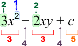
A coefficient is a numerical value, or letter representing a numerical constant, that multiplies a variable (the operator is omitted). A term is an addend or a summand, a group of coefficients, variables, constants and exponents that may be separated from the other terms by the plus and minus operators.[3] Letters represent variables and constants. By convention, letters at the beginning of the alphabet (e.g. ) are typically used to represent constants, and those toward the end of the alphabet (e.g. and z) are used to represent variables.[4] They are usually written in italics.[5]


Algebraic operations work in the same way as arithmetic operations,[6] such as addition, subtraction, multiplication, division and exponentiation.[7] and are applied to algebraic variables and terms. Multiplication symbols are usually omitted, and implied when there is no space between two variables or terms, or when a coefficient is used. For example, is written as , and may be written .[8]


Usually terms with the highest power (exponent), are written on the left, for example, is written to the left of x. When a coefficient is one, it is usually omitted (e.g. is written ).[9] Likewise when the exponent (power) is one, (e.g. is written ).[10] When the exponent is zero, the result is always 1 (e.g. is always rewritten to 1).[11] However , being undefined, should not appear in an expression, and care should be taken in simplifying expressions in which variables may appear in exponents.


Alternative notation
Other types of notation are used in algebraic expressions when the required formatting is not available, or can not be implied, such as where only letters and symbols are available. As an illustration of this, while exponents are usually formatted using superscripts, e.g., , in plain text, and in the TeX mark-up language, the caret symbol "^" represents exponentiation, so is written as "x^2".[12][13], as well as some programming languages such as Lua. In programming languages such as Ada,[14] Fortran,[15] Perl,[16] Python [17] and Ruby,[18] a double asterisk is used, so is written as "x**2". Many programming languages and calculators use a single asterisk to represent the multiplication symbol,[19] and it must be explicitly used, for example, is written "3*x".
Concepts
Variables

Elementary algebra builds on and extends arithmetic[20] by introducing letters called variables to represent general (non-specified) numbers. This is useful for several reasons.
- Variables may represent numbers whose values are not yet known. For example, if the temperature of the current day, C, is 20 degrees higher than the temperature of the previous day, P, then the problem can be described algebraically as .[21]
- Variables allow one to describe general problems,[22] without specifying the values of the quantities that are involved. For example, it can be stated specifically that 5 minutes is equivalent to seconds. A more general (algebraic) description may state that the number of seconds, , where m is the number of minutes.
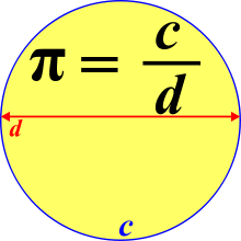
- Variables allow one to describe mathematical relationships between quantities that may vary.[23] For example, the relationship between the circumference, c, and diameter, d, of a circle is described by .
- Variables allow one to describe some mathematical properties. For example, a basic property of addition is commutativity which states that the order of numbers being added together does not matter. Commutativity is stated algebraically as .[24]


Simplifying expressions
Algebraic expressions may be evaluated and simplified, based on the basic properties of arithmetic operations (addition, subtraction, multiplication, division and exponentiation). For example,
- Added terms are simplified using coefficients. For example, can be simplified as (where 3 is a numerical coefficient).
- Multiplied terms are simplified using exponents. For example, is represented as
- Like terms are added together,[25] for example, is written as , because the terms containing are added together, and, the terms containing are added together.
- Brackets can be "multiplied out", using the distributive property. For example, can be written as which can be written as
- Expressions can be factored. For example, , by dividing both terms by can be written as


Equations
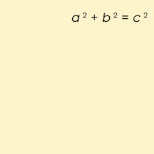
An equation states that two expressions are equal using the symbol for equality, = (the equals sign).[26] One of the best-known equations describes Pythagoras' law relating the length of the sides of a right angle triangle:[27]

This equation states that , representing the square of the length of the side that is the hypotenuse, the side opposite the right angle. That is equal to the sum (addition) of the squares of the other two sides whose lengths are represented by a and b.

An equation is the claim that two expressions have the same value and are equal. Some equations are true for all values of the involved variables (such as ); such equations are called identities. Conditional equations are true for only some values of the involved variables, e.g. is true only for and . The values of the variables which make the equation true are the solutions of the equation and can be found through equation solving.


Another type of equation is inequality. Inequalities are used to show that one side of the equation is greater, or less, than the other. The symbols used for this are: where represents 'greater than', and where represents 'less than'. Just like standard equality equations, numbers can be added, subtracted, multiplied or divided. The only exception is that when multiplying or dividing by a negative number, the inequality symbol must be flipped.


Properties of equality
By definition, equality is an equivalence relation, meaning it has the properties (a) reflexive (i.e. ), (b) symmetric (i.e. if then ) (c) transitive (i.e. if and then ).[28] It also satisfies the important property that if two symbols are used for equal things, then one symbol can be substituted for the other in any true statement about the first and the statement will remain true. This implies the following properties:


- if and then and ;
- if then and ;
- more generally, for any function f, if then .


Properties of inequality
The relations less than and greater than have the property of transitivity:[29]
- If and then ;
- If and then ;[30]
- If and then ;
- If and then .


By reversing the inequation, and can be swapped,[31] for example:
- is equivalent to

Substitution
Substitution is replacing the terms in an expression to create a new expression. Substituting 3 for a in the expression a*5 makes a new expression 3*5 with meaning 15. Substituting the terms of a statement makes a new statement. When the original statement is true independently of the values of the terms, the statement created by substitutions is also true. Hence, definitions can be made in symbolic terms and interpreted through substitution: if is meant as the definition of as the product of a with itself, substituting 3 for a informs the reader of this statement that means 3 × 3 = 9. Often it's not known whether the statement is true independently of the values of the terms. And, substitution allows one to derive restrictions on the possible values, or show what conditions the statement holds under. For example, taking the statement x + 1 = 0, if x is substituted with 1, this implies 1 + 1 = 2 = 0, which is false, which implies that if x + 1 = 0 then x cannot be 1.


If x and y are integers, rationals, or real numbers, then xy = 0 implies x = 0 or y = 0. Consider abc = 0. Then, substituting a for x and bc for y, we learn a = 0 or bc = 0. Then we can substitute again, letting x = b and y = c, to show that if bc = 0 then b = 0 or c = 0. Therefore, if abc = 0, then a = 0 or (b = 0 or c = 0), so abc = 0 implies a = 0 or b = 0 or c = 0.
If the original fact were stated as "ab = 0 implies a = 0 or b = 0", then when saying "consider abc = 0," we would have a conflict of terms when substituting. Yet the above logic is still valid to show that if abc = 0 then a = 0 or b = 0 or c = 0 if, instead of letting a = a and b = bc, one substitutes a for a and b for bc (and with bc = 0, substituting b for a and c for b). This shows that substituting for the terms in a statement isn't always the same as letting the terms from the statement equal the substituted terms. In this situation it's clear that if we substitute an expression a into the a term of the original equation, the a substituted does not refer to the a in the statement "ab = 0 implies a = 0 or b = 0."
Solving algebraic equations
The following sections lay out examples of some of the types of algebraic equations that may be encountered.
Linear equations with one variable
Linear equations are so-called, because when they are plotted, they describe a straight line. The simplest equations to solve are linear equations that have only one variable. They contain only constant numbers and a single variable without an exponent. As an example, consider:
- Problem in words: If you double the age of a child and add 4, the resulting answer is 12. How old is the child?
- Equivalent equation: where x represent the child's age

To solve this kind of equation, the technique is add, subtract, multiply, or divide both sides of the equation by the same number in order to isolate the variable on one side of the equation. Once the variable is isolated, the other side of the equation is the value of the variable.[32] This problem and its solution are as follows:
| 1. Equation to solve: | |
| 2. Subtract 4 from both sides: | |
| 3. This simplifies to: | |
| 4. Divide both sides by 2: | |
| 5. This simplifies to the solution: |


In words: the child is 4 years old.
The general form of a linear equation with one variable, can be written as:

Following the same procedure (i.e. subtract b from both sides, and then divide by a), the general solution is given by

Linear equations with two variables
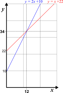
A linear equation with two variables has many (i.e. an infinite number of) solutions.[33] For example:
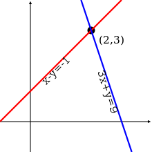
- Problem in words: A father is 22 years older than his son. How old are they?
- Equivalent equation: where y is the father's age, x is the son's age.

That cannot be worked out by itself. If the son's age was made known, then there would no longer be two unknowns (variables). The problem then becomes a linear equation with just one variable, that can be solved as described above.
To solve a linear equation with two variables (unknowns), requires two related equations. For example, if it was also revealed that:
- Problem in words
- In 10 years, the father will be twice as old as his son.
- Equivalent equation

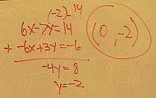
Now there are two related linear equations, each with two unknowns, which enables the production of a linear equation with just one variable, by subtracting one from the other (called the elimination method):[34]


In other words, the son is aged 12, and since the father 22 years older, he must be 34. In 10 years, the son will be 22, and the father will be twice his age, 44. This problem is illustrated on the associated plot of the equations.
For other ways to solve this kind of equations, see below, System of linear equations.
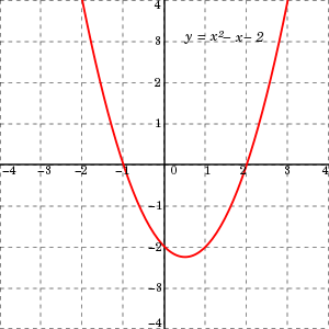
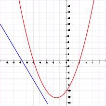
Quadratic equations
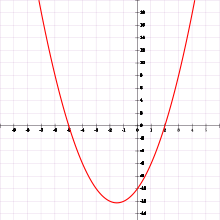


A quadratic equation is one which includes a term with an exponent of 2, for example, ,[35] and no term with higher exponent. The name derives from the Latin quadrus, meaning square.[36] In general, a quadratic equation can be expressed in the form ,[37] where a is not zero (if it were zero, then the equation would not be quadratic but linear). Because of this a quadratic equation must contain the term , which is known as the quadratic term. Hence , and so we may divide by a and rearrange the equation into the standard form


where and . Solving this, by a process known as completing the square, leads to the quadratic formula


where the symbol "±" indicates that both

are solutions of the quadratic equation.
Quadratic equations can also be solved using factorization (the reverse process of which is expansion, but for two linear terms is sometimes denoted foiling). As an example of factoring:

which is the same thing as

It follows from the zero-product property that either or are the solutions, since precisely one of the factors must be equal to zero. All quadratic equations will have two solutions in the complex number system, but need not have any in the real number system. For example,

has no real number solution since no real number squared equals −1. Sometimes a quadratic equation has a root of multiplicity 2, such as:

For this equation, −1 is a root of multiplicity 2. This means −1 appears twice, since the equation can be rewritten in factored form as

Complex numbers
All quadratic equations have exactly two solutions in complex numbers (but they may be equal to each other), a category that includes real numbers, imaginary numbers, and sums of real and imaginary numbers. Complex numbers first arise in the teaching of quadratic equations and the quadratic formula. For example, the quadratic equation

has solutions

Since is not any real number, both of these solutions for x are complex numbers.

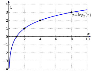
Exponential and logarithmic equations
An exponential equation is one which has the form for ,[38] which has solution


when . Elementary algebraic techniques are used to rewrite a given equation in the above way before arriving at the solution. For example, if


then, by subtracting 1 from both sides of the equation, and then dividing both sides by 3 we obtain

whence

or

A logarithmic equation is an equation of the form for , which has solution


For example, if

then, by adding 2 to both sides of the equation, followed by dividing both sides by 4, we get

whence

from which we obtain

Radical equations

A radical equation is one that includes a radical sign, which includes square roots, cube roots, , and nth roots, . Recall that an nth root can be rewritten in exponential format, so that is equivalent to . Combined with regular exponents (powers), then (the square root of x cubed), can be rewritten as .[39] So a common form of a radical equation is (equivalent to ) where m and n are integers. It has real solution(s):


| n is odd | n is even and |
n and m are even and |
n is even, m is odd, and |
|---|---|---|---|
|
equivalently |
equivalently |
no real solution |


For example, if:

then

and thus

System of linear equations
There are different methods to solve a system of linear equations with two variables.
Elimination method


An example of solving a system of linear equations is by using the elimination method:

Multiplying the terms in the second equation by 2:


Adding the two equations together to get:

which simplifies to

Since the fact that is known, it is then possible to deduce that by either of the original two equations (by using 2 instead of x ) The full solution to this problem is then


This is not the only way to solve this specific system; y could have been resolved before x.
Substitution method
Another way of solving the same system of linear equations is by substitution.
An equivalent for y can be deduced by using one of the two equations. Using the second equation:

Subtracting from each side of the equation:


and multiplying by −1:

Using this y value in the first equation in the original system:

Adding 2 on each side of the equation:

which simplifies to
Using this value in one of the equations, the same solution as in the previous method is obtained.
This is not the only way to solve this specific system; in this case as well, y could have been solved before x.
Other types of systems of linear equations
Inconsistent systems
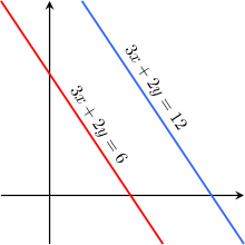


In the above example, a solution exists. However, there are also systems of equations which do not have any solution. Such a system is called inconsistent. An obvious example is

As 0≠2, the second equation in the system has no solution. Therefore, the system has no solution. However, not all inconsistent systems are recognized at first sight. As an example, consider the system

Multiplying by 2 both sides of the second equation, and adding it to the first one results in

which clearly has no solution.
Undetermined systems
There are also systems which have infinitely many solutions, in contrast to a system with a unique solution (meaning, a unique pair of values for x and y) For example:

Isolating y in the second equation:

And using this value in the first equation in the system:

The equality is true, but it does not provide a value for x. Indeed, one can easily verify (by just filling in some values of x) that for any x there is a solution as long as . There is an infinite number of solutions for this system.
Over- and underdetermined systems
Systems with more variables than the number of linear equations are called underdetermined. Such a system, if it has any solutions, does not have a unique one but rather an infinitude of them. An example of such a system is

When trying to solve it, one is led to express some variables as functions of the other ones if any solutions exist, but cannot express all solutions numerically because there are an infinite number of them if there are any.
A system with a higher number of equations than variables is called overdetermined. If an overdetermined system has any solutions, necessarily some equations are linear combinations of the others.
See also
- History of elementary algebra
- Binary operation
- Gaussian elimination
- Mathematics education
- Number line
- Polynomial
- Cancelling out
- Tarski's high school algebra problem
References
- Leonhard Euler, Elements of Algebra, 1770. English translation Tarquin Press, 2007, ISBN 978-1-899618-79-8, also online digitized editions[40] 2006,[41] 1822.
- Charles Smith, A Treatise on Algebra, in Cornell University Library Historical Math Monographs.
- Redden, John. Elementary Algebra. Flat World Knowledge, 2011
- H.E. Slaught and N.J. Lennes, Elementary algebra, Publ. Allyn and Bacon, 1915, page 1 (republished by Forgotten Books)
- Lewis Hirsch, Arthur Goodman, Understanding Elementary Algebra With Geometry: A Course for College Students, Publisher: Cengage Learning, 2005, ISBN 0534999727, 9780534999728, 654 pages, page 2
- Richard N. Aufmann, Joanne Lockwood, Introductory Algebra: An Applied Approach, Publisher Cengage Learning, 2010, ISBN 1439046042, 9781439046043, page 78
- William L. Hosch (editor), The Britannica Guide to Algebra and Trigonometry, Britannica Educational Publishing, The Rosen Publishing Group, 2010, ISBN 1615302190, 9781615302192, page 71
- James E. Gentle, Numerical Linear Algebra for Applications in Statistics, Publisher: Springer, 1998, ISBN 0387985425, 9780387985428, 221 pages, [James E. Gentle page 183]
- Horatio Nelson Robinson, New elementary algebra: containing the rudiments of science for schools and academies, Ivison, Phinney, Blakeman, & Co., 1866, page 7
- Ron Larson, Robert Hostetler, Bruce H. Edwards, Algebra And Trigonometry: A Graphing Approach, Publisher: Cengage Learning, 2007, ISBN 061885195X, 9780618851959, 1114 pages, page 6
- Sin Kwai Meng, Chip Wai Lung, Ng Song Beng, "Algebraic notation", in Mathematics Matters Secondary 1 Express Textbook, Publisher Panpac Education Pte Ltd, ISBN 9812738827, 9789812738820, page 68
- David Alan Herzog, Teach Yourself Visually Algebra, Publisher John Wiley & Sons, 2008, ISBN 0470185597, 9780470185599, 304 pages, page 72
- John C. Peterson, Technical Mathematics With Calculus, Publisher Cengage Learning, 2003, ISBN 0766861899, 9780766861893, 1613 pages, page 31
- Jerome E. Kaufmann, Karen L. Schwitters, Algebra for College Students, Publisher Cengage Learning, 2010, ISBN 0538733543, 9780538733540, 803 pages, page 222
- Ramesh Bangia, Dictionary of Information Technology, Publisher Laxmi Publications, Ltd., 2010, ISBN 9380298153, 9789380298153, page 212
- George Grätzer, First Steps in LaTeX, Publisher Springer, 1999, ISBN 0817641327, 9780817641320, page 17
- S. Tucker Taft, Robert A. Duff, Randall L. Brukardt, Erhard Ploedereder, Pascal Leroy, Ada 2005 Reference Manual, Volume 4348 of Lecture Notes in Computer Science, Publisher Springer, 2007, ISBN 3540693351, 9783540693352, page 13
- C. Xavier, Fortran 77 And Numerical Methods, Publisher New Age International, 1994, ISBN 812240670X, 9788122406702, page 20
- Randal Schwartz, Brian Foy, Tom Phoenix, Learning Perl, Publisher O'Reilly Media, Inc., 2011, ISBN 1449313140, 9781449313142, page 24
- Matthew A. Telles, Python Power!: The Comprehensive Guide, Publisher Course Technology PTR, 2008, ISBN 1598631586, 9781598631586, page 46
- Kevin C. Baird, Ruby by Example: Concepts and Code, Publisher No Starch Press, 2007, ISBN 1593271484, 9781593271480, page 72
- William P. Berlinghoff, Fernando Q. Gouvêa, Math through the Ages: A Gentle History for Teachers and Others, Publisher MAA, 2004, ISBN 0883857367, 9780883857366, page 75
- Thomas Sonnabend, Mathematics for Teachers: An Interactive Approach for Grades K-8, Publisher: Cengage Learning, 2009, ISBN 0495561665, 9780495561668, 759 pages, page xvii
- Lewis Hirsch, Arthur Goodman, Understanding Elementary Algebra With Geometry: A Course for College Students, Publisher: Cengage Learning, 2005, ISBN 0534999727, 9780534999728, 654 pages, page 48
- Lawrence S. Leff, College Algebra: Barron's Ez-101 Study Keys, Publisher: Barron's Educational Series, 2005, ISBN 0764129147, 9780764129148, 230 pages, page 2
- Ron Larson, Kimberly Nolting, Elementary Algebra, Publisher: Cengage Learning, 2009, ISBN 0547102275, 9780547102276, 622 pages, page 210
- Charles P. McKeague, Elementary Algebra, Publisher: Cengage Learning, 2011, ISBN 0840064217, 9780840064219, 571 pages, page 49
- Andrew Marx, Shortcut Algebra I: A Quick and Easy Way to Increase Your Algebra I Knowledge and Test Scores, Publisher Kaplan Publishing, 2007, ISBN 1419552880, 9781419552885, 288 pages, page 51
- Mark Clark, Cynthia Anfinson, Beginning Algebra: Connecting Concepts Through Applications, Publisher Cengage Learning, 2011, ISBN 0534419380, 9780534419387, 793 pages, page 134
- Alan S. Tussy, R. David Gustafson, Elementary and Intermediate Algebra, Publisher Cengage Learning, 2012, ISBN 1111567689, 9781111567682, 1163 pages, page 493
- Douglas Downing, Algebra the Easy Way, Publisher Barron's Educational Series, 2003, ISBN 0764119729, 9780764119729, 392 pages, page 20
- Ron Larson, Robert Hostetler, Intermediate Algebra, Publisher Cengage Learning, 2008, ISBN 0618753524, 9780618753529, 857 pages, page 96
- "What is the following property of inequality called?". Stack Exchange. November 29, 2014. Retrieved 4 May 2018.
- Chris Carter, Physics: Facts and Practice for A Level, Publisher Oxford University Press, 2001, ISBN 019914768X, 9780199147687, 144 pages, page 50
- Slavin, Steve (1989). All the Math You'll Ever Need. John Wiley & Sons. p. 72. ISBN 0-471-50636-2.
- Sinha, The Pearson Guide to Quantitative Aptitude for CAT 2/ePublisher: Pearson Education India, 2010, ISBN 8131723666, 9788131723661, 599 pages, page 195
- Cynthia Y. Young, Precalculus, Publisher John Wiley & Sons, 2010, ISBN 0471756849, 9780471756842, 1175 pages, page 699
- Mary Jane Sterling, Algebra II For Dummies, Publisher: John Wiley & Sons, 2006, ISBN 0471775819, 9780471775812, 384 pages, page 37
- John T. Irwin, The Mystery to a Solution: Poe, Borges, and the Analytic Detective Story, Publisher JHU Press, 1996, ISBN 0801854660, 9780801854668, 512 pages, page 372
- Sharma/khattar, The Pearson Guide To Objective Mathematics For Engineering Entrance Examinations, 3/E, Publisher Pearson Education India, 2010, ISBN 8131723631, 9788131723630, 1248 pages, page 621
- Aven Choo, LMAN OL Additional Maths Revision Guide 3, Publisher Pearson Education South Asia, 2007, ISBN 9810600011, 9789810600013, page 105
- John C. Peterson, Technical Mathematics With Calculus, Publisher Cengage Learning, 2003, ISBN 0766861899, 9780766861893, 1613 pages, page 525
- Euler's Elements of Algebra Archived 2011-04-13 at the Wayback Machine
- Euler, Leonhard; Hewlett, John; Horner, Francis; Bernoulli, Jean; Lagrange, Joseph Louis (4 May 2018). "Elements of Algebra". Longman, Orme. Retrieved 4 May 2018 – via Google Books.
External links

| Areas |
|
|---|---|
| Algebraic structures | |
| Linear algebra | |
| Multilinear algebra | |
| Topic lists | |
| Glossaries |
|
| Related | |
| |
| Foundations | |
|---|---|
| Algebra | |
| Analysis | |
| Discrete | |
| Geometry | |
| Number theory | |
| Topology | |
| Applied | |
| Computational | |
| Related topics | |
| |