Chebyshev polynomials

The Chebyshev polynomials are two sequences of polynomials, denoted T_n(x) and U_n(x). They are defined as follows. By the double angle formula,

\cos(2\theta )=2\cos ^{2}(\theta )-1

is a polynomial in cos(θ), so define T₂(x) = 2x² − 1. The other T_n(x) are defined similarly, using cos(nθ) = T_n(cos(θ)). Similarly, define the other sequence by sin(nθ) = U_n−1(cos(θ)) sin(θ), where we have used de Moivre's formula to note that sin(nθ) is sin(θ) times a polynomial in cos(θ). For instance,

\sin(3\theta )=(4\cos ^{2}(\theta )-1)\sin(\theta )

gives U₂(x) = 4x² − 1. The T_n(x) and U_n(x) are called Chebyshev polynomials of the first and second kind respectively.

The T_n(x) are orthogonal with respect to the inner product

{\big (}f(x),g(x){\big )}=\int _{-1}^{1}f(x)\,g(x)\,{\frac {dx}{\sqrt {1-x^{2}}}},

and U_n(x) are orthogonal with respect to a different product. This follows from the fact that the Chebyshev polynomials solve the Chebyshev differential equations

(1-x^{2})y''-xy'+n^{2}y=0,

(1-x^{2})y''-3xy'+n(n+2)y=0,

which are Sturm–Liouville differential equations. It is a general feature of such differential equations that there is a distinguished orthonormal set of solutions.

The Chebyshev polynomials T_n are polynomials with the largest possible leading coefficient whose absolute value on the interval $[-1, 1]$ is bounded by 1. They are also the extremal polynomials for many other properties.[1] Chebyshev polynomials are important in approximation theory because the roots of T_n(x), which are also called Chebyshev nodes, are used as nodes in polynomial interpolation. The resulting interpolation polynomial minimizes the problem of Runge's phenomenon and provides an approximation that is close to the polynomial of best approximation to a continuous function under the maximum norm. This approximation leads directly to the method of Clenshaw–Curtis quadrature.

These polynomials were named after Pafnuty Chebyshev.[2] The letter $T$ is used because of the alternative transliterations of the name Chebyshev as Tchebycheff, Tchebyshev (French) or Tschebyschow (German).

Definition

Plot of the first five Chebyshev

T

polynomials

Plot of the first five Chebyshev

U

polynomials

The Chebyshev polynomials of the first kind are defined by the recurrence relation

{\begin{aligned}T_{0}(x)&=1\\T_{1}(x)&=x\\T_{n+1}(x)&=2xT_{n}(x)-T_{n-1}(x).\end{aligned}}

The ordinary generating function for $T n$ is

\sum _{n=0}^{\infty }T_{n}(x)t^{n}={\frac {1-tx}{1-2tx+t^{2}}};

Proof

{\begin{aligned}G&=\sum _{n=0}^{\infty }T_{n}(x)t^{n}\\&=T_{0}(x)+tT_{1}(x)+\sum _{n=2}^{\infty }T_{n}(x)t^{n}\\&=1+tx+\sum _{n=0}^{\infty }T_{n+2}(x)t^{n+2}\\&=1+tx+\sum _{n=0}^{\infty }(2xT_{n+1}(x)-T_{n}(x))t^{n+2}\\&=1+tx+\sum _{n=0}^{\infty }2xT_{n+1}(x)t^{n+2}-\sum _{n=0}^{\infty }T_{n}(x)t^{n+2}\\&=1+tx+2tx\sum _{n=0}^{\infty }T_{n+1}(x)t^{n+1}-t^{2}\sum _{n=0}^{\infty }T_{n}(x)t^{n}\\&=1+tx+2tx(\sum _{n=0}^{\infty }T_{n}(x)t^{n}-1)-t^{2}\sum _{n=0}^{\infty }T_{n}(x)t^{n}\\&=1+tx+2tx(G-1)-t^{2}G\\&=1+tx+2txG-2tx-t^{2}G\\G-2txG+t^{2}G&=1+tx-2tx\\G&={\frac {1-tx}{1-2tx+t^{2}}}\end{aligned}}

the exponential generating function is

\sum _{n=0}^{\infty }T_{n}(x){\frac {t^{n}}{n!}}={\tfrac {1}{2}}\left(e^{\left(x-{\sqrt {x^{2}-1}}\right)t}+e^{\left(x+{\sqrt {x^{2}-1}}\right)t}\right)=e^{tx}\cosh \left(t{\sqrt {x^{2}-1}}\right).

The generating function relevant for 2-dimensional potential theory and multipole expansion is

\sum \limits _{n=1}^{\infty }T_{n}(x){\frac {t^{n}}{n}}=\ln {\frac {1}{\sqrt {1-2tx+t^{2}}}}.

The Chebyshev polynomials of the second kind are defined by the recurrence relation

{\begin{aligned}U_{0}(x)&=1\\U_{1}(x)&=2x\\U_{n+1}(x)&=2xU_{n}(x)-U_{n-1}(x).\end{aligned}}

The ordinary generating function for $U n$ is

\sum _{n=0}^{\infty }U_{n}(x)t^{n}={\frac {1}{1-2tx+t^{2}}};

the exponential generating function is

\sum _{n=0}^{\infty }U_{n}(x){\frac {t^{n}}{n!}}=e^{tx}\left(\cosh \left(t{\sqrt {x^{2}-1}}\right)+{\frac {x}{\sqrt {x^{2}-1}}}\sinh \left(t{\sqrt {x^{2}-1}}\right)\right).

Trigonometric definition

The Chebyshev polynomials of the first kind can be defined as the unique polynomials satisfying

T_{n}(x)={\begin{cases}\cos {\big (}n\arccos x{\big )},&{\text{if }}|x|\leq 1\\\cosh {\big (}n\operatorname {arcosh} x{\big )},&{\text{if }}x\geq 1\\(-1)^{n}\cosh {\big (}n\operatorname {arcosh} (-x){\big )},&{\text{if }}x\leq -1\end{cases}}

or, in other words, as the unique polynomials satisfying

T_{n}(\cos \theta )=\cos n\theta

for $n = 0, 1, 2, 3, ...$ which is a variant (equivalent transpose) of Schröder's equation, viz. $T n (x)$ is functionally conjugate to $nx$ , codified in the nesting property below. Further compare to the spread polynomials, in the section below.

The polynomials of the second kind satisfy:

U_{n-1}(\cos \theta )\cdot \sin \theta =\sin n\theta ,

or

U_{n}(\cos \theta )={\frac {\sin {\big (}(n{+}1)\theta {\big )}}{\sin \theta }},

which is structurally quite similar to the Dirichlet kernel $D n (x)$ :

D_{n}(x)={\frac {\sin \left((2n{+}1){\dfrac {x}{2}}\right)}{\sin {\dfrac {x}{2}}}}=U_{2n}\left(\cos {\frac {x}{2}}\right).

That $cos nx$ is an $n$ th-degree polynomial in $cos x$ can be seen by observing that $cos nx$ is the real part of one side of de Moivre's formula. The real part of the other side is a polynomial in $cos x$ and $sin x$ , in which all powers of $sin x$ are even and thus replaceable through the identity $cos 2 x + sin 2 x = 1$ . By the same reasoning, $sin nx$ is the imaginary part of the polynomial, in which all powers of $sin x$ are odd and thus, if one is factored out, the remaining can be replaced to create a $(n-1)$ th-degree polynomial in $cos x$ .

The identity is quite useful in conjunction with the recursive generating formula, inasmuch as it enables one to calculate the cosine of any integral multiple of an angle solely in terms of the cosine of the base angle.

Evaluating the first two Chebyshev polynomials,

T_{0}(\cos \theta )=\cos 0\theta =1

and

T_{1}(\cos \theta )=\cos \theta ,

one can straightforwardly determine that

{\begin{aligned}\cos 2\theta &=2\cos \theta \cos \theta -1=2\cos ^{2}\theta -1\\\cos 3\theta &=2\cos \theta \cos 2\theta -\cos \theta =4\cos ^{3}\theta -3\cos \theta ,\end{aligned}}

and so forth.

Two immediate corollaries are the composition identity (or nesting property specifying a semigroup)

T_{n}{\big (}T_{m}(x){\big )}=T_{nm}(x);

and the expression of complex exponentiation in terms of Chebyshev polynomials: given $z = a + bi$ ,

{\begin{aligned}z^{n}&=|z|^{n}\left(\cos \left(n\arccos {\frac {a}{|z|}}\right)+i\sin \left(n\arccos {\frac {a}{|z|}}\right)\right)\\&=|z|^{n}T_{n}\left({\frac {a}{|z|}}\right)+ib|z|^{n-1}\ U_{n-1}\left({\frac {a}{|z|}}\right).\end{aligned}}

Pell equation definition

The Chebyshev polynomials can also be defined as the solutions to the Pell equation

T_{n}(x)^{2}-\left(x^{2}-1\right)U_{n-1}(x)^{2}=1

in a ring $R [x]$ .[3] Thus, they can be generated by the standard technique for Pell equations of taking powers of a fundamental solution:

T_{n}(x)+U_{n-1}(x){\sqrt {x^{2}-1}}=(x+{\sqrt {x^{2}-1}})^{n}.

Products of Chebyshev polynomials

When working with Chebyshev polynomials quite often products of two of them occur. These products can be reduced to combinations of Chebyshev polynomials with lower or higher degree and concluding statements about the product are easier to make. It shall be assumed that in the following the index m is greater than or equal to the index n and n is not negative. For Chebyshev polynomials of the first kind the product expands to

2T_{m}(x)T_{n}(x)=T_{m+n}(x)+T_{|m-n|}(x)

which is an analogy to the addition theorem

2\cos \alpha \cos \beta =\cos(\alpha +\beta )+\cos(\alpha -\beta )

with the identities

\alpha =m\arccos x,\beta =n\arccos x.

For $n = 1$ this results in the already known recurrence formula, just arranged differently, and with $n = 2$ it forms the recurrence relation for all even or all odd Chebyshev polynomials (depending on the parity of the lowest $m$ ) which allows to design functions with prescribed symmetry properties. Three more useful formulas for evaluating Chebyshev polynomials can be concluded from this product expansion:

{\begin{aligned}T_{2n}(x)&=2T_{n}^{2}(x)-T_{0}(x)&&=2T_{n}^{2}(x)-1\\T_{2n+1}(x)&=2T_{n+1}(x)T_{n}(x)-T_{1}(x)&&=2T_{n+1}(x)T_{n}(x)-x\\T_{2n-1}(x)&=2T_{n-1}(x)T_{n}(x)-T_{1}(x)&&=2T_{n-1}(x)T_{n}(x)-x\end{aligned}}

For Chebyshev polynomials of the second kind, products may be written as:

U_{m}(x)U_{n}(x)=\sum _{k=0}^{n}U_{m-n+2k}(x)=\sum _{\underset {\text{step 2}}{p=m-n}}^{m+n}U_{p}(x).

for $m \geq n$ .

By this, like above, with $n = 2$ the recurrence formula for Chebyshev polynomials of the second kind reduces for both types of symmetry to

U_{m+2}(x)=U_{2}(x)U_{m}(x)-U_{m}(x)-U_{m-2}(x)=U_{m}(x){\big (}U_{2}(x)-1{\big )}-U_{m-2}(x),

depending on whether $m$ starts with 2 or 3.

Relations between Chebyshev polynomials of the first and second kinds

The Chebyshev polynomials of the first and second kinds correspond to a complementary pair of Lucas sequences $Ṽ n (P, Q)$ and $Ũ n (P, Q)$ with parameters $P = 2 x$ and $Q = 1$ :

{\begin{aligned}{\tilde {U}}_{n}(2x,1)&=U_{n-1}(x),\\{\tilde {V}}_{n}(2x,1)&=2\cdot T_{n}(x).\end{aligned}}

It follows that they also satisfy a pair of mutual recurrence equations:

{\begin{aligned}T_{n+1}(x)&=xT_{n}(x)-(1-x^{2})U_{n-1}(x),\\U_{n}(x)&=xU_{n-1}(x)+T_{n}(x).\end{aligned}}

The Chebyshev polynomials of the first and second kinds are also connected by the following relations:

{\begin{aligned}T_{n}(x)&={\tfrac {1}{2}}{\big (}U_{n}(x)-U_{n-2}(x){\big )}.&&\\T_{n}(x)&=U_{n}(x)-x\,U_{n-1}(x).&&\\U_{n}(x)&=2\sum _{{\text{odd }}j}^{n}T_{j}(x)&&{\text{for odd }}n.\\U_{n}(x)&=2\sum _{{\text{even }}j}^{n}T_{j}(x)-1&&{\text{for even }}n.\end{aligned}}

The recurrence relationship of the derivative of Chebyshev polynomials can be derived from these relations:

2T_{n}(x)={\frac {1}{n+1}}\,{\frac {d}{dx}}T_{n+1}(x)-{\frac {1}{n-1}}\,{\frac {d}{dx}}T_{n-1}(x)\qquad n=2,3,\ldots

This relationship is used in the Chebyshev spectral method of solving differential equations.

Turán's inequalities for the Chebyshev polynomials are

{\begin{aligned}T_{n}(x)^{2}-T_{n-1}(x)T_{n+1}(x)&=1-x^{2}>0&&{\text{for }}-1<x<1&&{\text{and}}\\U_{n}(x)^{2}-U_{n-1}(x)U_{n+1}(x)&=1>0.\end{aligned}}

The integral relations are

{\begin{aligned}\int _{-1}^{1}{\frac {T_{n}(y)dy}{(y-x){\sqrt {1-y^{2}}}}}&=\pi U_{n-1}(x),\\\int _{-1}^{1}{\frac {{\sqrt {1-y^{2}}}U_{n-1}(y)dy}{y-x}}&=-\pi T_{n}(x)\end{aligned}}

where integrals are considered as principal value.

Explicit expressions

Different approaches to defining Chebyshev polynomials lead to different explicit expressions such as:

{\begin{aligned}T_{n}(x)&={\begin{cases}\cos(n\arccos x)&|x|\leq 1\\\\{\frac {1}{2}}{\bigg (}{\Big (}x-{\sqrt {x^{2}-1}}{\Big )}^{n}+{\Big (}x+{\sqrt {x^{2}-1}}{\Big )}^{n}{\bigg )}\qquad &|x|\geq 1\\\end{cases}}\\\\\\&={\begin{cases}\cos(n\arccos x)&-1\leq x\leq 1\\\\\cosh(n\operatorname {arcosh} x)&1\leq x\\(-1)^{n}\cosh {\big (}n\operatorname {arcosh} (-x){\big )}\qquad &x\leq -1\\\end{cases}}\\\\\\T_{n}(x)&=\sum _{k=0}^{\left\lfloor {\frac {n}{2}}\right\rfloor }{\binom {n}{2k}}\left(x^{2}-1\right)^{k}x^{n-2k}\\&=x^{n}\sum _{k=0}^{\left\lfloor {\frac {n}{2}}\right\rfloor }{\binom {n}{2k}}\left(1-x^{-2}\right)^{k}\\&={\tfrac {n}{2}}\sum _{k=0}^{\left\lfloor {\frac {n}{2}}\right\rfloor }(-1)^{k}{\frac {(n-k-1)!}{k!(n-2k)!}}~(2x)^{n-2k}\qquad n>0\\&=n\sum _{k=0}^{n}(-2)^{k}{\frac {(n+k-1)!}{(n-k)!(2k)!}}(1-x)^{k}\qquad n>0\\&={}_{2}F_{1}\left(-n,n;{\tfrac {1}{2}};{\tfrac {1}{2}}(1-x)\right)\\\end{aligned}}

with inverse[4][5]

x^{n}=2^{1-n}\mathop {{\sum }'} _{j=0,n-j\mathrm {even} }^{n}{\binom {n}{\tfrac {n-j}{2}}}T_{j}(x),

where the prime at the sum symbol indicates that the contribution of $j = 0$ needs to be halved if it appears.

{\begin{aligned}U_{n}(x)&={\frac {\left(x+{\sqrt {x^{2}-1}}\right)^{n+1}-\left(x-{\sqrt {x^{2}-1}}\right)^{n+1}}{2{\sqrt {x^{2}-1}}}}\\&=\sum _{k=0}^{\left\lfloor {\frac {n}{2}}\right\rfloor }{\binom {n+1}{2k+1}}\left(x^{2}-1\right)^{k}x^{n-2k}\\&=x^{n}\sum _{k=0}^{\left\lfloor {\frac {n}{2}}\right\rfloor }{\binom {n+1}{2k+1}}\left(1-x^{-2}\right)^{k}\\&=\sum _{k=0}^{\left\lfloor {\frac {n}{2}}\right\rfloor }{\binom {2k-(n+1)}{k}}~(2x)^{n-2k}&&n>0\\&=\sum _{k=0}^{\left\lfloor {\frac {n}{2}}\right\rfloor }(-1)^{k}{\binom {n-k}{k}}~(2x)^{n-2k}&&n>0\\&=\sum _{k=0}^{n}(-2)^{k}{\frac {(n+k+1)!}{(n-k)!(2k+1)!}}(1-x)^{k}&&n>0\\&=(n+1)\ {}_{2}F_{1}\left(-n,n+2;{\tfrac {3}{2}};{\tfrac {1}{2}}(1-x)\right)\\\end{aligned}}

where $2 F 1$ is a hypergeometric function.

Properties

Symmetry

{\begin{aligned}T_{n}(-x)&=(-1)^{n}T_{n}(x)\\&={\begin{cases}T_{n}(x),&n{\text{ even}}\\-T_{n}(x),&n{\text{ odd}}\end{cases}}\\U_{n}(-x)&=(-1)^{n}U_{n}(x)\\&={\begin{cases}U_{n}(x),&n{\text{ even}}\\-U_{n}(x),&n{\text{ odd}}\end{cases}}\\\end{aligned}}

That is, Chebyshev polynomials of even order have even symmetry and contain only even powers of $x$ . Chebyshev polynomials of odd order have odd symmetry and contain only odd powers of $x$ .

Roots and extrema

A Chebyshev polynomial of either kind with degree $n$ has $n$ different simple roots, called Chebyshev roots, in the interval $[-1,1]$ . The roots of the Chebyshev polynomial of the first kind are sometimes called Chebyshev nodes because they are used as nodes in polynomial interpolation. Using the trigonometric definition and the fact that

\cos \left((2k+1){\frac {\pi }{2}}\right)=0

one can show that the roots of $T n$ are

x_{k}=\cos \left({\frac {\pi (k+1/2)}{n}}\right),\quad k=0,\ldots ,n-1.

Similarly, the roots of $U n$ are

x_{k}=\cos \left({\frac {k}{n+1}}\pi \right),\quad k=1,\ldots ,n.

The extrema of $T n$ on the interval $-1 \leq x \leq 1$ are located at

x_{k}=\cos \left({\frac {k}{n}}\pi \right),\quad k=0,\ldots ,n.

One unique property of the Chebyshev polynomials of the first kind is that on the interval $-1 \leq x \leq 1$ all of the extrema have values that are either −1 or 1. Thus these polynomials have only two finite critical values, the defining property of Shabat polynomials. Both the first and second kinds of Chebyshev polynomial have extrema at the endpoints, given by:

T_{n}(1)=1

T_{n}(-1)=(-1)^{n}

U_{n}(1)=n+1

U_{n}(-1)=(n+1)(-1)^{n}.

Differentiation and integration

The derivatives of the polynomials can be less than straightforward. By differentiating the polynomials in their trigonometric forms, it can be shown that:

{\begin{aligned}{\frac {dT_{n}}{dx}}&=nU_{n-1}\\{\frac {dU_{n}}{dx}}&={\frac {(n+1)T_{n+1}-xU_{n}}{x^{2}-1}}\\{\frac {d^{2}T_{n}}{dx^{2}}}&=n{\frac {nT_{n}-xU_{n-1}}{x^{2}-1}}=n{\frac {(n+1)T_{n}-U_{n}}{x^{2}-1}}.\end{aligned}}

The last two formulas can be numerically troublesome due to the division by zero (0/0 indeterminate form, specifically) at $x = 1$ and $x = -1$ . It can be shown that:

{\begin{aligned}\left.{\frac {d^{2}T_{n}}{dx^{2}}}\right|_{x=1}\!\!&={\frac {n^{4}-n^{2}}{3}},\\\left.{\frac {d^{2}T_{n}}{dx^{2}}}\right|_{x=-1}\!\!&=(-1)^{n}{\frac {n^{4}-n^{2}}{3}}.\end{aligned}}

Proof

The second derivative of the Chebyshev polynomial of the first kind is

T''_{n}=n{\frac {nT_{n}-xU_{n-1}}{x^{2}-1}}

which, if evaluated as shown above, poses a problem because it is indeterminate at $x = \pm1$ . Since the function is a polynomial, (all of) the derivatives must exist for all real numbers, so the taking to limit on the expression above should yield the desired value:

T''_{n}(1)=\lim _{x\to 1}n{\frac {nT_{n}-xU_{n-1}}{x^{2}-1}}

where only $x = 1$ is considered for now. Factoring the denominator:

T''_{n}(1)=\lim _{x\to 1}n{\frac {nT_{n}-xU_{n-1}}{(x+1)(x-1)}}=\lim _{x\to 1}n{\frac {\;{\dfrac {nT_{n}-xU_{n-1}}{x-1}}\;}{x+1}}.

Since the limit as a whole must exist, the limit of the numerator and denominator must independently exist, and

T''_{n}(1)=n{\frac {\displaystyle {\lim _{x\to 1}}{\frac {nT_{n}-xU_{n-1}}{x-1}}}{\displaystyle {\lim _{x\to 1}}(x+1)}}={\frac {n}{2}}\lim _{x\to 1}{\frac {nT_{n}-xU_{n-1}}{x-1}}.

The denominator (still) limits to zero, which implies that the numerator must be limiting to zero, i.e. $U n - 1 (1) = nT n (1) = n$ which will be useful later on. Since the numerator and denominator are both limiting to zero, L'Hôpital's rule applies:

{\begin{aligned}T''_{n}(1)&={\frac {n}{2}}\lim _{x\to 1}{\frac {{\frac {d}{dx}}(nT_{n}-xU_{n-1})}{{\frac {d}{dx}}(x-1)}}\\&={\frac {n}{2}}\lim _{x\to 1}{\frac {d}{dx}}(nT_{n}-xU_{n-1})\\&={\frac {n}{2}}\lim _{x\to 1}\left(n^{2}U_{n-1}-U_{n-1}-x{\frac {d}{dx}}(U_{n-1})\right)\\&={\frac {n}{2}}\left(n^{2}U_{n-1}(1)-U_{n-1}(1)-\lim _{x\to 1}x{\frac {d}{dx}}(U_{n-1})\right)\\&={\frac {n^{4}}{2}}-{\frac {n^{2}}{2}}-{\frac {1}{2}}\lim _{x\to 1}{\frac {d}{dx}}(nU_{n-1})\\&={\frac {n^{4}}{2}}-{\frac {n^{2}}{2}}-{\frac {T''_{n}(1)}{2}}\\T''_{n}(1)&={\frac {n^{4}-n^{2}}{3}}.\\\end{aligned}}

The proof for $x = -1$ is similar, with the fact that $T n (-1) = (-1) n$ being important.

Indeed, the following, more general formula holds:

\left.{\frac {d^{p}T_{n}}{dx^{p}}}\right|_{x=\pm 1}\!\!=(\pm 1)^{n+p}\prod _{k=0}^{p-1}{\frac {n^{2}-k^{2}}{2k+1}}.

This latter result is of great use in the numerical solution of eigenvalue problems.

{\frac {d^{p}}{dx^{p}}}T_{n}(x)=2^{p}n\mathop {{\sum }'} _{k\geq 0,n-p-k\mathrm {even} }^{n-p}{\binom {{\frac {n+p-k}{2}}-1}{\frac {n-p-k}{2}}}{\frac {\left({\frac {n+p+k}{2}}-1\right)!}{\left({\frac {n-p+k}{2}}\right)!}}T_{k}(x),\qquad p\geq 1,

where the prime at the summation symbols means that the term contributed by $k = 0$ is to be halved, if it appears.

Concerning integration, the first derivative of the $T n$ implies that

\int U_{n}\,dx={\frac {T_{n+1}}{n+1}}

and the recurrence relation for the first kind polynomials involving derivatives establishes that for $n \geq 2$

\int T_{n}\,dx={\frac {1}{2}}\left({\frac {T_{n+1}}{n+1}}-{\frac {T_{n-1}}{n-1}}\right)={\frac {nT_{n+1}}{n^{2}-1}}-{\frac {xT_{n}}{n-1}}.

and

\int _{-1}^{1}T_{n}(x)\,dx={\begin{cases}{\frac {(-1)^{n}+1}{1-n^{2}}}&n\neq 1\\0&n=1\end{cases}}

Orthogonality

Both $T n$ and $U n$ form a sequence of orthogonal polynomials. The polynomials of the first kind $T n$ are orthogonal with respect to the weight

{\frac {1}{\sqrt {1-x^{2}}}},

on the interval $[-1,1]$ , i.e. we have:

\int _{-1}^{1}T_{n}(x)T_{m}(x)\,{\frac {dx}{\sqrt {1-x^{2}}}}={\begin{cases}0&{\text{if }}n\neq m,\\\pi &{\text{if }}n=m=0,\\{\frac {\pi }{2}}&{\text{if }}n=m\neq 0.\end{cases}}

This can be proven by letting $x = cos θ$ and using the defining identity $T n (cos θ) = cos nθ$ .

Similarly, the polynomials of the second kind $U n$ are orthogonal with respect to the weight

{\sqrt {1-x^{2}}}

on the interval $[-1,1]$ , i.e. we have:

\int _{-1}^{1}U_{n}(x)U_{m}(x){\sqrt {1-x^{2}}}\,dx={\begin{cases}0&{\text{if }}n\neq m,\\{\frac {\pi }{2}}&{\text{if }}n=m.\end{cases}}

(The measure $\sqrt 1 - x 2 dx$ is, to within a normalizing constant, the Wigner semicircle distribution.)

The $T n$ also satisfy a discrete orthogonality condition:

\sum _{k=0}^{N-1}{T_{i}(x_{k})T_{j}(x_{k})}={\begin{cases}0&{\text{if }}i\neq j,\\N&{\text{if }}i=j=0,\\{\frac {N}{2}}&{\text{if }}i=j\neq 0,\end{cases}}

where $N$ is any integer greater than $i + j$ , and the $x k$ are the $N$ Chebyshev nodes (see above) of $T N (x)$ :

x_{k}=\cos \left(\pi {\frac {2k+1}{2N}}\right),\quad k=0,1,\dots ,N-1.

For the polynomials of the second kind and any integer $N > i + j$ with the same Chebyshev nodes $x k$ , there are similar sums:

\sum _{k=0}^{N-1}{U_{i}(x_{k})U_{j}(x_{k})\left(1-x_{k}^{2}\right)}={\begin{cases}0&{\text{if }}i\neq j,\\{\frac {N}{2}}&{\text{if }}i=j,\end{cases}}

and without the weight function:

\sum _{k=0}^{N-1}{U_{i}(x_{k})U_{j}(x_{k})}={\begin{cases}0&{\text{if }}i\not \equiv j{\pmod {2}},\\N\cdot (1+\min(i,j))&{\text{if }}i\equiv j{\pmod {2}}.\end{cases}}

For any integer $N > i + j$ , based on the $N$ zeros of $U N (x)$ :

y_{k}=\cos \left(\pi {\frac {k+1}{N+1}}\right),\quad k=0,1,\dots ,N-1,

one can get the sum:

\sum _{k=0}^{N-1}{U_{i}(y_{k})U_{j}(y_{k})(1-y_{k}^{2})}={\begin{cases}0&{\text{if }}i\neq j,\\{\frac {N+1}{2}}&{\text{if }}i=j,\end{cases}}

and again without the weight function:

\sum _{k=0}^{N-1}{U_{i}(y_{k})U_{j}(y_{k})}={\begin{cases}0&{\text{if }}i\not \equiv j{\pmod {2}},\\{\big (}\min(i,j)+1{\big )}{\big (}N-\max(i,j){\big )}&{\text{if }}i\equiv j{\pmod {2}}.\end{cases}}

Minimal $\infty$ -norm

For any given $n \geq 1$ , among the polynomials of degree $n$ with leading coefficient 1 (monic polynomials),

f(x)={\frac {1}{2^{n-1}}}T_{n}(x)

is the one of which the maximal absolute value on the interval [−1, 1] is minimal.

This maximal absolute value is

{\frac {1}{2^{n-1}}}

and $| f (x) |$ reaches this maximum exactly $n + 1$ times at

x=\cos {\frac {k\pi }{n}}\quad {\text{for }}0\leq k\leq n.

Proof

Let's assume that $w n (x)$ is a polynomial of degree $n$ with leading coefficient 1 with maximal absolute value on the interval $[-1,1]$ less than $1 / 2 n - 1$ .

Define

f_{n}(x)={\frac {1}{2^{n-1}}}T_{n}(x)-w_{n}(x)

Because at extreme points of $T n$ we have

{\begin{aligned}|w_{n}(x)|&<\left|{\frac {1}{2^{n-1}}}T_{n}(x)\right|\\f_{n}(x)&>0\qquad {\text{for }}x=\cos {\frac {2k\pi }{n}}&&{\text{where }}0\leq 2k\leq n\\f_{n}(x)&<0\qquad {\text{for }}x=\cos {\frac {(2k+1)\pi }{n}}&&{\text{where }}0\leq 2k+1\leq n\end{aligned}}

From the intermediate value theorem, $f n (x)$ has at least $n$ roots. However, this is impossible, as $f n (x)$ is a polynomial of degree $n - 1$ , so the fundamental theorem of algebra implies it has at most $n - 1$ roots.

Remark: By the Equioscillation theorem, among all the polynomials of degree $\leq n$ , the polynomial $f$ minimizes $| | f | | \infty$ on $[-1,1]$ if and only if there are $n + 2$ points $-1 \leq x 0 < x 1 < ... < x n + 1 \leq 1$ such that $| f (x i) | = | | f | | \infty$ .

Of course, the null polynomial on the interval $[-1,1]$ can be approach by itself and minimizes the $\infty$ -norm.

Above, however, $| f |$ reaches its maximum only $n + 1$ times because we are searching for the best polynomial of degree $n \geq 1$ (therefore the theorem evoked previously cannot be used).

Other properties

The Chebyshev polynomials are a special case of the ultraspherical or Gegenbauer polynomials, which themselves are a special case of the Jacobi polynomials:

{\begin{aligned}T_{n}(x)&={\frac {n}{2}}\lim _{q\to 0}{\frac {1}{q}}C_{n}^{(q)}(x)\qquad {\text{if }}n\geq 1,\\U_{n}(x)&={\frac {n+1}{n+{\frac {1}{2}} \choose n}}P_{n}^{({\frac {1}{2}},{\frac {1}{2}})}(x)={\frac {n+1}{n+{\frac {1}{2}} \choose n}}C_{n}^{(1)}(x).\end{aligned}}

For every nonnegative integer $n$ , $T n (x)$ and $U n (x)$ are both polynomials of degree $n$ . They are even or odd functions of $x$ as $n$ is even or odd, so when written as polynomials of $x$ , it only has even or odd degree terms respectively. In fact,

T_{2n}(x)=T_{n}\left(2x^{2}-1\right)=2T_{n}(x)^{2}-1

and

2xU_{n}\left(1-2x^{2}\right)=(-1)^{n}U_{2n+1}(x).

The leading coefficient of $T n$ is $2 n - 1$ if $1 \leq n$ , but 1 if $0 = n$ .

$T n$ are a special case of Lissajous curves with frequency ratio equal to $n$ .

Several polynomial sequences like Lucas polynomials ( $L n$ ), Dickson polynomials ( $D n$ ), Fibonacci polynomials ( $F n$ ) are related to Chebyshev polynomials $T n$ and $U n$ .

The Chebyshev polynomials of the first kind satisfy the relation

T_{j}(x)T_{k}(x)={\tfrac {1}{2}}\left(T_{j+k}(x)+T_{|k-j|}(x)\right),\qquad \forall j,k\geq 0,\,

which is easily proved from the product-to-sum formula for the cosine. The polynomials of the second kind satisfy the similar relation

T_{j}(x)U_{k}(x)={\begin{cases}{\tfrac {1}{2}}\left(U_{j+k}(x)+U_{k-j}(x)\right),&{\text{if }}k\geq j-1.\\{\tfrac {1}{2}}\left(U_{j+k}(x)-U_{j-k-2}(x)\right),&{\text{if }}k\leq j-2.\end{cases}}

(with the convention $U -1 \equiv 0$ ).

Similar to the formula

T_{n}(\cos \theta )=\cos n\theta ,

we have the analogous formula

T_{2n+1}(\sin \theta )=(-1)^{n}\sin {\big (}(2n+1)\theta {\big )}

.

For $x \neq 0$ ,

T_{n}\left({\frac {x+x^{-1}}{2}}\right)={\frac {x^{n}+x^{-n}}{2}}

and

x^{n}=T_{n}\left({\frac {x+x^{-1}}{2}}\right)+{\frac {x-x^{-1}}{2}}U_{n-1}\left({\frac {x+x^{-1}}{2}}\right)

,

which follows from the fact that this holds by definition for $x = e iθ$ .

Let

C_{n}(x)=2T_{n}\left({\frac {x}{2}}\right)

.

Then $C n (x)$ and $C m (x)$ are commuting polynomials:

C_{n}{\big (}C_{m}(x){\big )}=C_{m}{\big (}C_{n}(x){\big )}

,

as is evident in the Abelian nesting property specified above.

Generalized Chebyshev polynomials

The generalized Chebyshev polynomials T_a are defined by

T_{a}(\cos x)={}_{2}F_{1}\left(a,-a;{\tfrac {1}{2}};{\tfrac {1}{2}}(1-\cos x)\right)=\cos ax,\qquad x\in (-\pi ,\pi ),

where $a$ is not necessarily an integer, and $2 F 1 (a, b; c; z)$ is the Gaussian hypergeometric function; as an example $T_{1/2}(x)={\sqrt {\frac {1+x}{2}}}$ . The power series expansion

T_{a}(x)=\cos \left({\frac {\pi a}{2}}\right)+a\sum _{j=1}{\frac {(2x)^{j}}{2j}}\cos \left({\frac {\pi (a-j)}{2}}\right){{\frac {a+j-2}{2}} \choose j-1}

converges for $x\in [-1,1]$ .

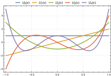
Examples

First kind

The first few Chebyshev polynomials of the first kind in the domain

-1 < x < 1

: The flat

T 0

,

T 1

,

T 2

,

T 3

,

T 4

and

T 5

.

The first few Chebyshev polynomials of the first kind are OEIS: A028297

{\begin{aligned}T_{0}(x)&=1\\T_{1}(x)&=x\\T_{2}(x)&=2x^{2}-1\\T_{3}(x)&=4x^{3}-3x\\T_{4}(x)&=8x^{4}-8x^{2}+1\\T_{5}(x)&=16x^{5}-20x^{3}+5x\\T_{6}(x)&=32x^{6}-48x^{4}+18x^{2}-1\\T_{7}(x)&=64x^{7}-112x^{5}+56x^{3}-7x\\T_{8}(x)&=128x^{8}-256x^{6}+160x^{4}-32x^{2}+1\\T_{9}(x)&=256x^{9}-576x^{7}+432x^{5}-120x^{3}+9x\\T_{10}(x)&=512x^{10}-1280x^{8}+1120x^{6}-400x^{4}+50x^{2}-1\\T_{11}(x)&=1024x^{11}-2816x^{9}+2816x^{7}-1232x^{5}+220x^{3}-11x\end{aligned}}

Second kind

The first few Chebyshev polynomials of the second kind in the domain

-1 < x < 1

: The flat

U 0

,

U 1

,

U 2

,

U 3

,

U 4

and

U 5

. Although not visible in the image,

U n (1) = n + 1

and

U n (-1) = (n + 1)(-1) n

.

The first few Chebyshev polynomials of the second kind are OEIS: A053117

{\begin{aligned}U_{0}(x)&=1\\U_{1}(x)&=2x\\U_{2}(x)&=4x^{2}-1\\U_{3}(x)&=8x^{3}-4x\\U_{4}(x)&=16x^{4}-12x^{2}+1\\U_{5}(x)&=32x^{5}-32x^{3}+6x\\U_{6}(x)&=64x^{6}-80x^{4}+24x^{2}-1\\U_{7}(x)&=128x^{7}-192x^{5}+80x^{3}-8x\\U_{8}(x)&=256x^{8}-448x^{6}+240x^{4}-40x^{2}+1\\U_{9}(x)&=512x^{9}-1024x^{7}+672x^{5}-160x^{3}+10x\end{aligned}}

As a basis set

The non-smooth function (top)

y = - x 3 H (- x)

, where

H

is the Heaviside step function, and (bottom) the 5th partial sum of its Chebyshev expansion. The 7th sum is indistinguishable from the original function at the resolution of the graph.

In the appropriate Sobolev space, the set of Chebyshev polynomials form an orthonormal basis, so that a function in the same space can, on $-1 \leq x \leq 1$ be expressed via the expansion:[6]

f(x)=\sum _{n=0}^{\infty }a_{n}T_{n}(x).

Furthermore, as mentioned previously, the Chebyshev polynomials form an orthogonal basis which (among other things) implies that the coefficients $a n$ can be determined easily through the application of an inner product. This sum is called a Chebyshev series or a Chebyshev expansion.

Since a Chebyshev series is related to a Fourier cosine series through a change of variables, all of the theorems, identities, etc. that apply to Fourier series have a Chebyshev counterpart.[6] These attributes include:

The Chebyshev polynomials form a complete orthogonal system.
The Chebyshev series converges to $f (x)$ if the function is piecewise smooth and continuous. The smoothness requirement can be relaxed in most cases — as long as there are a finite number of discontinuities in $f (x)$ and its derivatives.
At a discontinuity, the series will converge to the average of the right and left limits.

The abundance of the theorems and identities inherited from Fourier series make the Chebyshev polynomials important tools in numeric analysis; for example they are the most popular general purpose basis functions used in the spectral method,[6] often in favor of trigonometric series due to generally faster convergence for continuous functions (Gibbs' phenomenon is still a problem).

Example 1

Consider the Chebyshev expansion of $log(1 + x)$ . One can express

\log(1+x)=\sum _{n=0}^{\infty }a_{n}T_{n}(x).

One can find the coefficients $a n$ either through the application of an inner product or by the discrete orthogonality condition. For the inner product,

\int _{-1}^{+1}{\frac {T_{m}(x)\log(1+x)}{\sqrt {1-x^{2}}}}\,dx=\sum _{n=0}^{\infty }a_{n}\int _{-1}^{+1}{\frac {T_{m}(x)T_{n}(x)}{\sqrt {1-x^{2}}}}\,dx,

which gives

a_{n}={\begin{cases}-\log 2&n=0\\{\frac {-2(-1)^{n}}{n}}&n>0.\end{cases}}

Alternatively, when the inner product of the function being approximated cannot be evaluated, the discrete orthogonality condition gives an often useful result for approximate coefficients,

a_{n}\approx {\frac {2-\delta _{0n}}{N}}\sum _{k=0}^{N-1}T_{n}(x_{k})\log(1+x_{k}),

where $δ ij$ is the Kronecker delta function and the $x k$ are the $N$ Gauss–Chebyshev zeros of $T N (x)$ :

x_{k}=\cos \left({\frac {\pi \left(k+{\frac {1}{2}}\right)}{N}}\right).

For any $N$ , these approximate coefficients provide an exact approximation to the function at $x k$ with a controlled error between those points. The exact coefficients are obtained with $N = \infty$ , thus representing the function exactly at all points in $[-1,1]$ . The rate of convergence depends on the function and its smoothness.

This allows us to compute the approximate coefficients $a n$ very efficiently through the discrete cosine transform

a_{n}\approx {\frac {2-\delta _{0n}}{N}}\sum _{k=0}^{N-1}\cos \left({\frac {n\pi \left(k+{\frac {1}{2}}\right)}{N}}\right)\log(1+x_{k}).

Example 2

To provide another example:

{\begin{aligned}(1-x^{2})^{\alpha }=&-{\frac {1}{\sqrt {\pi }}}{\frac {\Gamma \left({\frac {1}{2}}+\alpha \right)}{\Gamma (\alpha +1)}}+2^{1-2\alpha }\sum _{n=0}(-1)^{n}{2\alpha  \choose \alpha -n}T_{2n}(x)\\=&2^{-2\alpha }\sum _{n=0}(-1)^{n}{2\alpha +1 \choose \alpha -n}U_{2n}(x).\end{aligned}}

Partial sums

The partial sums of

f(x)=\sum _{n=0}^{\infty }a_{n}T_{n}(x)

are very useful in the approximation of various functions and in the solution of differential equations (see spectral method). Two common methods for determining the coefficients $a n$ are through the use of the inner product as in Galerkin's method and through the use of collocation which is related to interpolation.

As an interpolant, the $N$ coefficients of the $(N - 1)$ th partial sum are usually obtained on the Chebyshev–Gauss–Lobatto[7] points (or Lobatto grid), which results in minimum error and avoids Runge's phenomenon associated with a uniform grid. This collection of points corresponds to the extrema of the highest order polynomial in the sum, plus the endpoints and is given by:

x_{k}=-\cos \left({\frac {k\pi }{N-1}}\right);\qquad k=0,1,\dots ,N-1.

Polynomial in Chebyshev form

An arbitrary polynomial of degree $N$ can be written in terms of the Chebyshev polynomials of the first kind.[8] Such a polynomial $p (x)$ is of the form

p(x)=\sum _{n=0}^{N}a_{n}T_{n}(x).

Polynomials in Chebyshev form can be evaluated using the Clenshaw algorithm.

Shifted Chebyshev polynomials

Shifted Chebyshev polynomials of the first kind are defined as

T_{n}^{*}(x)=T_{n}(2x-1).

When the argument of the Chebyshev polynomial is in the range of $2 x - 1 \in [-1,1]$ the argument of the shifted Chebyshev polynomial is $x \in [0,1]$ . Similarly, one can define shifted polynomials for generic intervals $[a, b]$ .

Spread polynomials

The spread polynomials are a rescaling of the shifted Chebyshev polynomials of the first kind so that the range is also $[0,1]$ . That is,

S_{n}(x)={\frac {1-T_{n}(1-2x)}{2}}.

Notes

Rivlin, Theodore J. The Chebyshev polynomials. Pure and Applied Mathematics. Wiley-Interscience [John Wiley & Sons], New York-London-Sydney, 1974. Chapter 2, "Extremal Properties", pp. 56–123.
Chebyshev polynomials were first presented in: Chebyshev, P. L. (1854). "Théorie des mécanismes connus sous le nom de parallélogrammes". Mémoires des Savants étrangers présentés à l'Académie de Saint-Pétersbourg (in French). 7: 539–586.
Jeroen Demeyer Diophantine Sets over Polynomial Rings and Hilbert's Tenth Problem for Function Fields Archived 2007-07-02 at the Wayback Machine, Ph.D. theses (2007), p.70.
Cody, W. J. (1970). "A survey of practical rational and polynomial approximation of functions". SIAM Review. 12 (3). pp. 400–423. doi:10.1137/1012082.
Mathar, R. J. (2006). "Chebyshev series expansion of inverse polynomials". J. Comput. Appl. Math. 196 (2): 596–607. arXiv:math/0403344. Bibcode:2006JCoAM..196.596M. doi:10.1016/j.cam.2005.10.013.
Boyd, John P. (2001). Chebyshev and Fourier Spectral Methods (PDF) (second ed.). Dover. ISBN 0-486-41183-4. Archived from the original (PDF) on 2010-03-31. Retrieved 2009-03-19.
Chebyshev Interpolation: An Interactive Tour
For more information on the coefficients, see: Mason, J. C. and Handscomb, D. C. (2002). Chebyshev Polynomials. Taylor & Francis.

References

Abramowitz, Milton; Stegun, Irene Ann, eds. (1983) [June 1964]. "Chapter 22". Handbook of Mathematical Functions with Formulas, Graphs, and Mathematical Tables. Applied Mathematics Series. 55 (Ninth reprint with additional corrections of tenth original printing with corrections (December 1972); first ed.). Washington D.C.; New York: United States Department of Commerce, National Bureau of Standards; Dover Publications. p. 773. ISBN 978-0-486-61272-0. LCCN 64-60036. MR 0167642. LCCN 65-12253.
Dette, Holger (1995). "A Note on Some Peculiar Nonlinear Extremal Phenomena of the Chebyshev Polynomials". Proceedings of the Edinburgh Mathematical Society. 38 (2): 343–355. arXiv:math/9406222. doi:10.1017/S001309150001912X.
Elliott, David (1964). "The evaluation and estimation of the coefficients in the Chebyshev Series expansion of a function". Math. Comp. 18 (86): 274–284. doi:10.1090/S0025-5718-1964-0166903-7. MR 0166903.
Eremenko, A.; Lempert, L. (1994). "An Extremal Problem For Polynomials" (PDF). Proceedings of the American Mathematical Society. 122 (1): 191–193. doi:10.1090/S0002-9939-1994-1207536-1. MR 1207536.
Hernandez, M. A. (2001). "Chebyshev's approximation algorithms and applications". Comp. Math. Applic. 41 (3–4): 433–445. doi:10.1016/s0898-1221(00)00286-8.
Mason, J. C. (1984). "Some properties and applications of Chebyshev polynomial and rational approximation". Lect. Not. Math. Lecture Notes in Mathematics. 1105: 27–48. doi:10.1007/BFb0072398. ISBN 978-3-540-13899-0.
Mason, J. C.; Handscomb, D. C. (2002). Chebyshev Polynomials. Taylor & Francis.
Mathar, R. J. (2006). "Chebyshev series expansion of inverse polynomials". J. Comput. Appl. Math. 196 (2): 596–607. arXiv:math/0403344. Bibcode:2006JCoAM.196..596M. doi:10.1016/j.cam.2005.10.013.
Koornwinder, Tom H.; Wong, Roderick S. C.; Koekoek, Roelof; Swarttouw, René F. (2010), "Orthogonal Polynomials", in Olver, Frank W. J.; Lozier, Daniel M.; Boisvert, Ronald F.; Clark, Charles W. (eds.), NIST Handbook of Mathematical Functions, Cambridge University Press, ISBN 978-0-521-19225-5, MR 2723248
Remes, Eugene. "On an Extremal Property of Chebyshev Polynomials" (PDF).
Salzer, Herbert E. (1976). "Converting interpolation series into Chebyshev Series by Recurrence Formulas". Math. Comp. 30 (134): 295–302. doi:10.1090/S0025-5718-1976-0395159-3. MR 0395159.
Scraton, R. E. (1969). "The Solution of integral equations in Chebyshev series". Math. Comput. 23 (108): 837–844. doi:10.1090/S0025-5718-1969-0260224-4. MR 0260224.
Smith, Lyle B. (1966). "Algorithm 277, Computation of Chebyshev series coefficients". Comm. ACM. 9 (2): 86–87. doi:10.1145/365170.365195.
Suetin, P. K. (2001) [1994], "C/c021940", in Hazewinkel, Michiel (ed.), Encyclopedia of Mathematics, Springer Science+Business Media B.V. / Kluwer Academic Publishers, ISBN 978-1-55608-010-4

External links

Weisstein, Eric W. "Chebyshev Polynomial of the First Kind". MathWorld.
Module for Chebyshev Polynomials by John H. Mathews
Chebyshev Interpolation: An Interactive Tour, includes illustrative Java applet.
Numerical Computing with Functions: The Chebfun Project
Is there an intuitive explanation for an extremal property of Chebyshev polynomials?
Chebyshev polynomial evaluation and the Chebyshev transform in Boost.Math

This article is issued from Wikipedia. The text is licensed under Creative Commons - Attribution - Sharealike. Additional terms may apply for the media files.

[1] Rivlin, Theodore J. The Chebyshev polynomials. Pure and Applied Mathematics. Wiley-Interscience [John Wiley & Sons], New York-London-Sydney, 1974. Chapter 2, "Extremal Properties", pp. 56–123.

[2] Chebyshev polynomials were first presented in: Chebyshev, P. L. (1854). "Théorie des mécanismes connus sous le nom de parallélogrammes". Mémoires des Savants étrangers présentés à l'Académie de Saint-Pétersbourg (in French). 7: 539–586.

[3] Jeroen Demeyer Diophantine Sets over Polynomial Rings and Hilbert's Tenth Problem for Function Fields Archived 2007-07-02 at the Wayback Machine, Ph.D. theses (2007), p.70.

[Cody-4] Cody, W. J. (1970). "A survey of practical rational and polynomial approximation of functions". SIAM Review. 12 (3). pp. 400–423. doi:10.1137/1012082.

[Mathar-5] Mathar, R. J. (2006). "Chebyshev series expansion of inverse polynomials". J. Comput. Appl. Math. 196 (2): 596–607. arXiv:math/0403344. Bibcode:2006JCoAM..196.596M. doi:10.1016/j.cam.2005.10.013.

[boyd-6] Boyd, John P. (2001). Chebyshev and Fourier Spectral Methods (PDF) (second ed.). Dover. ISBN 0-486-41183-4. Archived from the original (PDF) on 2010-03-31. Retrieved 2009-03-19.

[7] Chebyshev Interpolation: An Interactive Tour

[8] For more information on the coefficients, see: Mason, J. C. and Handscomb, D. C. (2002). Chebyshev Polynomials. Taylor & Francis.

Chebyshev polynomials

Definition

Trigonometric definition

Pell equation definition

Products of Chebyshev polynomials

Relations between Chebyshev polynomials of the first and second kinds

Explicit expressions

Properties

Symmetry

Roots and extrema

Differentiation and integration

Orthogonality

Minimal ∞-norm

Other properties

Generalized Chebyshev polynomials

Examples

First kind

Second kind

As a basis set

Example 1

Example 2

Partial sums

Polynomial in Chebyshev form

Shifted Chebyshev polynomials

Spread polynomials

See also

Notes

References

External links

Minimal $\infty$ -norm