Upsampling

In digital signal processing, upsampling can refer to the entire process of increasing the sampling rate of a signal, or it can refer to just one step of the process, the other step being interpolation. Complementary to decimation, which decreases sampling rate, it is a specific case of sample rate conversion in a multi-rate digital signal processing system. When upsampling is performed on a sequence of samples of a signal or other continuous function, it produces an approximation of the sequence that would have been obtained by sampling the signal at a higher rate (or density, as in the case of a photograph). For example, if compact disc audio at 44,100 samples/second is upsampled by a factor of 5/4, the resulting sample-rate is 55,125.

Upsampling by an integer factor

Rate increase by an integer factor L can be explained as a 2-step process, with an equivalent implementation that is more efficient:

Create a sequence, $\scriptstyle x_{L}[n],$ comprising the original samples, $\scriptstyle x[n],$ separated by L − 1 zeros. This alone is sometimes referred to as upsampling.
Interpolation: Smooth out the discontinuities with a lowpass filter, which replaces the zeros.

In this application, the filter is called an interpolation filter, and its design is discussed below. When the interpolation filter is an FIR type, its efficiency can be improved, because the zeros contribute nothing to its dot product calculations. It is an easy matter to omit them from both the data stream and the calculations. The calculation performed by an efficient interpolating FIR filter for each output sample is a dot product:

y[j+nL]=\sum _{k=0}^{K}x[n-k]\cdot h[j+kL],\ \ j=0,1,\ldots ,L-1,

where the h[•] sequence is the impulse response, and K is the largest value of k for which h[j + kL] is non-zero. In the case L = 2, h[•] can be designed as a half-band filter, where almost half of the coefficients are zero and need not be included in the dot products. Impulse response coefficients taken at intervals of L form a subsequence, and there are L such subsequences (called phases) multiplexed together. Each of L phases of the impulse response is filtering the same sequential values of the x[•] data stream and producing one of L sequential output values. In some multi-processor architectures, these dot products are performed simultaneously, in which case it is called a polyphase filter.

For completeness, we now mention that a possible, but unlikely, implementation of each phase is to replace the coefficients of the other phases with zeros in a copy of the h[•] array, and process the $\scriptstyle x_{L}[n]$ sequence at L times faster than the original input rate. Then L-1 of every L outputs are zero. The desired y[•] sequence is the sum of the phases, where L-1 terms of the each sum are identically zero. Computing L-1 zeros between the useful outputs of a phase and adding them to a sum is effectively decimation. It's the same result as not computing them at all. That equivalence is known as the second Noble identity.^[1]

Fig 1: Spectral depictions of zero-fill and interpolation by lowpass filtering

Interpolation filter design

Let X(f) be the Fourier transform of any function, x(t), whose samples at some interval, T, equal the x[n] sequence. Then the discrete-time Fourier transform (DTFT) of the x[n] sequence is the Fourier series representation of a periodic summation of X(f):

$\underbrace {\sum _{n=-\infty }^{\infty }\overbrace {x(nT)} ^{x[n]}\ e^{-i2\pi fnT}} _{\text{DTFT}}={\frac {1}{T}}\sum _{k=-\infty }^{\infty }X(f-k/T).$

(Eq.1)

When T has units of seconds, $\scriptstyle f$ has units of hertz. Sampling L times faster (at interval T/L) increases the periodicity by a factor of L:

${\frac {L}{T}}\sum _{k=-\infty }^{\infty }X\left(f-k\cdot {\frac {L}{T}}\right),$

(Eq.2)

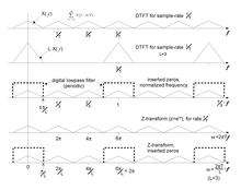
which is also the desired result of interpolation. An example of both these distributions is depicted in the top two graphs of Fig.1.

When the additional samples are inserted zeros, they increase the data rate, but they have no effect on the frequency distribution until the zeros are replaced by the interpolation filter. Many filter design programs use frequency units of cycles/sample, which is achieved by normalizing the frequency axis, based on the new data rate (L/T). The result is shown in the third graph of Fig.1. Also shown is the passband of the interpolation filter needed to make the third graph resemble the second one. Its cutoff frequency is ${\tfrac {0.5}{L}}.$ ^{[note 1]} In terms of actual frequency, the cutoff is ${\tfrac {0.5}{T}}$ Hz, which is the Nyquist frequency of the original x[n] sequence.

The same result can be obtained from Z-transforms, constrained to values of complex-variable, z, of the form $z=e^{i\omega }.$ Then the transform is the same Fourier series with different frequency normalization. By comparison with Eq.1, we deduce:

\sum _{n=-\infty }^{\infty }x[n]\ z^{-n}=\sum _{n=-\infty }^{\infty }x[n]\ e^{-i\omega n}={\frac {1}{T}}\sum _{k=-\infty }^{\infty }\underbrace {X\left({\tfrac {\omega }{2\pi T}}-{\tfrac {k}{T}}\right)} _{X\left({\frac {\omega -2\pi k}{2\pi T}}\right)},

which is depicted by the fourth graph in Fig.1. When the zeros are inserted, the transform becomes:

\sum _{n=-\infty }^{\infty }x[n]\ z^{-nL}=\sum _{n=-\infty }^{\infty }x[n]\ e^{-i\omega Ln}={\frac {1}{T}}\sum _{k=-\infty }^{\infty }\underbrace {X\left({\tfrac {\omega L}{2\pi T}}-{\tfrac {k}{T}}\right)} _{X\left({\frac {\omega -2\pi k/L}{2\pi T/L}}\right)},

depicted by the bottom graph. In these normalizations, the effective data-rate is always represented by the constant 2 $π$ (radians/sample) instead of 1. In those units, the interpolation filter bandwidth is $π$ /L, as show on the bottom graph. The corresponding physical frequency is ${\tfrac {\pi }{L}}\cdot {\tfrac {L}{2\pi T}}={\tfrac {0.5}{T}}$ Hz, the original Nyquist frequency.

Upsampling by a rational fraction

Let L/M denote the upsampling factor, where L > M.

Upsample by a factor of L
Decimate by a factor of M

Upsampling requires a lowpass filter after increasing the data rate, and decimation requires a lowpass filter before downsampling. Therefore, both operations can be accomplished by a single filter with the lower of the two cutoff frequencies. For the L > M case, the interpolation filter cutoff, ${\tfrac {0.5}{L}}$ cycles per intermediate sample, is the lower frequency.

Notes

↑ Realizable low-pass filters have a "skirt", where the response diminishes from near unity to near zero. So in practice the cutoff frequency is placed far enough below the theoretical cutoff that the filter's skirt is contained below the theoretical cutoff.

Citations

↑ Strang, Gilbert; Nguyen, Truong (1996-10-01). Wavelets and Filter Banks (2 ed.). Wellesley,MA: Wellesley-Cambridge Press. pp. 100–101. ISBN 0961408871.

References

Oppenheim, Alan V.; Schafer, Ronald W.; Buck, John R. (1999). Discrete-Time Signal Processing (2nd ed.). Prentice Hall. ISBN 0-13-754920-2.
Tan, Li (2008-04-21). "Upsampling and downsampling". eetimes.com. EE Times. Retrieved 2017-04-10.
"Digital Audio Resampling Home Page". (discusses a technique for bandlimited interpolation)
"Matlab example of using polyphase filters for interpolation".

This article is issued from Wikipedia. The text is licensed under Creative Commons - Attribution - Sharealike. Additional terms may apply for the media files.

[2] Realizable low-pass filters have a "skirt", where the response diminishes from near unity to near zero. So in practice the cutoff frequency is placed far enough below the theoretical cutoff that the filter's skirt is contained below the theoretical cutoff.

[Strang-1] Strang, Gilbert; Nguyen, Truong (1996-10-01). Wavelets and Filter Banks (2 ed.). Wellesley,MA: Wellesley-Cambridge Press. pp. 100–101. ISBN 0961408871.

Digital signal processing
Theory	Detection theory Discrete signal Estimation theory Nyquist–Shannon sampling theorem
Sub-fields	Audio signal processing Digital image processing Speech processing Statistical signal processing
Techniques	Advanced Z-transform Bilinear transform Constant-Q transform Discrete Fourier transform (DFT) Discrete-time Fourier transform (DTFT) Impulse invariance Integral transform Laplace transform Matched Z-transform method Post's inversion formula Starred transform Z-transform Zak transform
Sampling	Aliasing Anti-aliasing filter Downsampling Nyquist rate / frequency Oversampling Quantization Sampling rate Undersampling Upsampling