Stress–strain curve
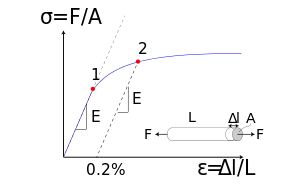


1: Elastic (proportionality) limit
2: Offset yield strength (0.2% proof strength)
The relationship between the stress and strain that a particular material displays is known as that particular material's stress–strain curve. It is unique for each material and is found by recording the amount of deformation (strain) at distinct intervals of tensile or compressive loading (stress). These curves reveal many of the properties of a material (including data to establish the Modulus of Elasticity, E).[1]
Stress–strain curves of various materials vary widely, and different tensile tests conducted on the same material yield different results, depending upon the temperature of the specimen and the speed of the loading. It is possible, however, to distinguish some common characteristics among the stress–strain curves of various groups of materials and, on this basis, to divide materials into two broad categories; namely, the ductile materials and the brittle materials.[2]
Consider a bar of cross sectional area A being subjected to equal and opposite forces F pulling at the ends so the bar is under tension. The material is experiencing a stress defined to be the ratio of the force to the cross sectional area of the bar:

Note that for engineering purposes, we often assume the cross-section area of the material does not change during the whole deformation process, which is not true since the actual area will decrease while deforming due to elastic and plastic deformation. The one assuming cross-section area fixed is so called “engineering stress-strain curve”, the latter is “true stress-strain curve”. In a tension test, true strain is less than engineering strain. Thus, a point defining true stress-strain curve is displaced upwards and to the left to define the equivalent engineering stress-strain curve. The difference between the true and engineering stresses and strains will increase with plastic deformation. At low strains (such as elastic deformation), the differences between the two is negligible.
Two important effects necessary to understand the true stress are the effects of strain rate susceptibility and strain rate hardening upon the true stress. Time is often neglected in the initial stress-strain curve relations, but at higher strain rates, higher stresses will occur according to the relationship σT=k'ἕTm where m is the strain rate susceptibility. To account for the resistance to necking, the relationship σT=kεTn must also be considered, where n is the strain hardening coefficient and is typically between 0.02 and 0.50, depending upon the material. By combining these two relationships, a relationship of σT=kεTnἕTm can be found. However, as real stresses and strains do not occur uniaxially, considerations for multiaxial stresses must be added to this relationship to model real stresses.
This stress is called the tensile stress because every part of the object is subjected to tension. The SI unit of stress is the newton per square meter, which is called the pascal.
1 pascal = 1 Pa = 1 N/m2
Now consider a force that is applied tangentially to an object. The ratio of the shearing force to the area A is called the shear stress.
If the object is twisted through an angle q, then the shear strain is:

Finally, the shear modulus MS of a material is defined as the ratio of shear stress to shear strain at any point in an object made of that material. The shear modulus is also known as the torsion modulus.
Ductile materials

- 1: Ultimate strength
- 2: Yield strength (yield point)
- 3: Rupture
- 4: Strain hardening region
- 5: Necking region
- A: Apparent stress (F/A0)
- B: Actual stress (F/A)
Ductile materials, which includes structural steel and many alloys of other metals, are characterized by their ability to yield at normal temperatures.[3]
Low carbon steel generally exhibits a very linear stress–strain relationship up to a well defined yield point (Fig.2). The linear portion of the curve is the elastic region and the slope is the modulus of elasticity or Young's Modulus ( Young's Modulus is the ratio of the compressive stress to the longitudinal strain). Many ductile materials including some metals, polymers and ceramics exhibit a yield point. Plastic flow initiates at the upper yield point and continues at the lower one. At lower yield point, permanent deformation is heterogeneously distributed along the sample. The deformation band which formed at the upper yield point will propagate along the gauge length at the lower yield point. The band occupies the whole of the gauge at the luders strain. Beyond this point, work hardening commences. The appearance of the yield point is associated with pinning of dislocations in the system. Specifically, solid solution interacts with dislocations and acts as pin and prevent dislocation from moving. Therefore, the stress needed to initiate the movement will be large. As long as the dislocation escape from the pinning, stress needed to continue it is less.
After the yield point, the curve typically decreases slightly because of dislocations escaping from Cottrell atmospheres. As deformation continues, the stress increases on account of strain hardening until it reaches the ultimate tensile stress. Until this point, the cross-sectional area decreases uniformly and randomly because of Poisson contractions. The actual fracture point is in the same vertical line as the visual fracture point.
However, beyond this point a neck forms where the local cross-sectional area becomes significantly smaller than the original. If the specimen is subjected to progressively increasing tensile force it reaches the ultimate tensile stress and then necking and elongation occur rapidly until fracture. If the specimen is subjected to progressively increasing length it is possible to observe the progressive necking and elongation, and to measure the decreasing tensile force in the specimen.
The appearance of necking in ductile materials is associated with geometrical instability in the system. Due to the natural inhomogeneity of the material, it is common to find some regions with small inclusions or porosity within it or surface, where strain will concentrate, leading to a locally smaller area than other regions. For strain less than the ultimate tensile strain, the increase of work-hardening rate in this region will be greater than the area reduction rate, thereby make this region harder to be further deform than others, so that the instability will be removed, i.e. the materials have abilities to weaken the inhomogeneity before reaching ultimate strain. However, as the strain become larger, the work hardening rate will decreases, so that for now the region with smaller area is weaker than other region, therefore reduction in area will concentrate in this region and the neck becomes more and more pronounced until fracture. After the neck has formed in the materials, further plastic deformation is concentrated in the neck while the remainder of the material undergoes elastic contraction owing to the decrease in tensile force.
The stress-strain curve for a ductile material can be approximated using the Ramberg-Osgood equation.[4] This equation is straightforward to implement, and only requires the material's yield strength, ultimate strength, elastic modulus, and percent elongation.
Brittle materials
Brittle materials, which includes cast iron, glass, and stone, are characterized by the fact that rupture occurs without any noticeable prior change in the rate of elongation.[5]
Brittle materials such as concrete or carbon fiber do not have a yield point, and do not strain-harden. Therefore, the ultimate strength and breaking strength are the same. A typical stress–strain curve is shown in Fig.3. Typical brittle materials like glass do not show any plastic deformation but fail while the deformation is elastic. One of the characteristics of a brittle failure is that the two broken parts can be reassembled to produce the same shape as the original component as there will not be a neck formation like in the case of ductile materials. A typical stress–strain curve for a brittle material will be linear. For some materials, such as concrete, tensile strength is negligible compared to the compressive strength and it is assumed zero for many engineering applications. Glass fibers have a tensile strength stronger than steel, but bulk glass usually does not. This is because of the stress intensity factor associated with defects in the material. As the size of the sample gets larger, the size of defects also grows. In general, the tensile strength of a rope is always less than the sum of the tensile strengths of its individual fibers.
See also
References
- ↑ Luebkeman, C., & Peting, D. (2012, 04 28). Stress–strain curves. Retrieved from http://pages.uoregon.edu/struct/courseware/461/461_lectures/461_lecture24/461_lecture24.html.
- ↑ Beer, F, Johnston, R, Dewolf, J, & Mazurek, D. (2009). Mechanics of materials. New York: McGraw-Hill companies. P 51.
- ↑ Beer, F, Johnston, R, Dewolf, J, & Mazurek, D. (2009). Mechanics of materials. New York: McGraw-Hill companies. P 58.
- ↑ "Mechanical Properties of Materials".
- ↑ Beer, F, Johnston, R, Dewolf, J, & Mazurek, D. (2009). Mechanics of materials. New York: McGraw-Hill companies. P 59.