Dijkstra's algorithm

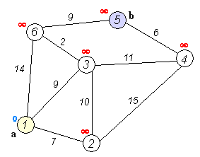Dijkstra's algorithm
	Dijkstra's algorithm to find the shortest path between a and b. It picks the unvisited vertex with the lowest distance, calculates the distance through it to each unvisited neighbor, and updates the neighbor's distance if smaller. Mark visited (set to red) when done with neighbors.
Class	Search algorithm
Data structure	Graph
Worst-case performance

Dijkstra's algorithm is an algorithm for finding the shortest paths between nodes in a graph, which may represent, for example, road networks. It was conceived by Dutch computer scientist Edsger W. Dijkstra in 1956 and published three years later.^[1]^[2]^[3]

The algorithm exists in many variants; Dijkstra's original variant found the shortest path between two nodes,^[3] but a more common variant fixes a single node as the "source" node and finds shortest paths from the source to all other nodes in the graph, producing a shortest-path tree.

For a given source node in the graph, the algorithm finds the shortest path between that node and every other.^[4]^:196–206 It can also be used for finding the shortest paths from a single node to a single destination node by stopping the algorithm once the shortest path to the destination node has been determined. For example, if the nodes of the graph represent cities and edge path costs represent driving distances between pairs of cities connected by a direct road, Dijkstra's algorithm can be used to find the shortest route between one city and all other cities. As a result, the shortest path algorithm is widely used in network routing protocols, most notably IS-IS (Intermediate System to Intermediate System) and Open Shortest Path First (OSPF). It is also employed as a subroutine in other algorithms such as Johnson's.

Dijkstra's original algorithm does not use a min-priority queue and runs in time $O(|V|^{2})$ (where $|V|$ is the number of nodes). The idea of this algorithm is also given in Leyzorek et al. 1957. The implementation based on a min-priority queue implemented by a Fibonacci heap and running in $O(|E|+|V|\log |V|)$ (where $|E|$ is the number of edges) is due to Fredman & Tarjan 1984. This is asymptotically the fastest known single-source shortest-path algorithm for arbitrary directed graphs with unbounded non-negative weights. However, specialized cases (such as bounded/integer weights, directed acyclic graphs etc.) can indeed be improved further as detailed in § Specialized variants.

In some fields, artificial intelligence in particular, Dijkstra's algorithm or a variant of it is known as uniform cost search and formulated as an instance of the more general idea of best-first search.^[5]

History

What is the shortest way to travel from Rotterdam to Groningen, in general: from given city to given city. It is the algorithm for the shortest path, which I designed in about twenty minutes. One morning I was shopping in Amsterdam with my young fiancée, and tired, we sat down on the café terrace to drink a cup of coffee and I was just thinking about whether I could do this, and I then designed the algorithm for the shortest path. As I said, it was a twenty-minute invention. In fact, it was published in ’59, three years late. The publication is still readable, it is, in fact, quite nice. One of the reasons that it is so nice was that I designed it without pencil and paper. I learned later that one of the advantages of designing without pencil and paper is that you are almost forced to avoid all avoidable complexities. Eventually that algorithm became, to my great amazement, one of the cornerstones of my fame.
— Edsger Dijkstra, in an interview with Philip L. Frana, Communications of the ACM, 2001^[2]

Dijkstra thought about the shortest path problem when working at the Mathematical Center in Amsterdam in 1956 as a programmer to demonstrate the capabilities of a new computer called ARMAC.^[6] His objective was to choose both a problem and a solution (that would be produced by computer) that non-computing people could understand. He designed the shortest path algorithm and later implemented it for ARMAC for a slightly simplified transportation map of 64 cities in the Netherlands (64, so that 6 bits would be sufficient to encode the city number).^[2] A year later, he came across another problem from hardware engineers working on the institute's next computer: minimize the amount of wire needed to connect the pins on the back panel of the machine. As a solution, he re-discovered the algorithm known as Prim's minimal spanning tree algorithm (known earlier to Jarník, and also rediscovered by Prim).^[7]^[8] Dijkstra published the algorithm in 1959, two years after Prim and 29 years after Jarník.^[9]^[10]

Algorithm

Illustration of Dijkstra's algorithm finding a path from a start node (lower left, red) to a goal node (upper right, green) in a robot motion planning problem. Open nodes represent the "tentative" set (aka set of "unvisited" nodes). Filled nodes are visited ones, with color representing the distance: the greener, the closer. Nodes in all the different directions are explored uniformly, appearing more-or-less as a circular wavefront as Dijkstra's algorithm uses a heuristic identically equal to 0.

Let the node at which we are starting be called the initial node. Let the distance of node Y be the distance from the initial node to Y. Dijkstra's algorithm will assign some initial distance values and will try to improve them step by step.

Mark all nodes unvisited. Create a set of all the unvisited nodes called the unvisited set.
Assign to every node a tentative distance value: set it to zero for our initial node and to infinity for all other nodes. Set the initial node as current.
For the current node, consider all of its unvisited neighbors and calculate their tentative distances through the current node. Compare the newly calculated tentative distance to the current assigned value and assign the smaller one. For example, if the current node A is marked with a distance of 6, and the edge connecting it with a neighbor B has length 2, then the distance to B through A will be 6 + 2 = 8. If B was previously marked with a distance greater than 8 then change it to 8. Otherwise, keep the current value.
When we are done considering all of the unvisited neighbors of the current node, mark the current node as visited and remove it from the unvisited set. A visited node will never be checked again.
If the destination node has been marked visited (when planning a route between two specific nodes) or if the smallest tentative distance among the nodes in the unvisited set is infinity (when planning a complete traversal; occurs when there is no connection between the initial node and remaining unvisited nodes), then stop. The algorithm has finished.
Otherwise, select the unvisited node that is marked with the smallest tentative distance, set it as the new "current node", and go back to step 3.

When planning a route, it is actually not necessary to wait until the destination node is "visited" as above: the algorithm can stop once the destination node has the smallest tentative distance among all "unvisited" nodes (and thus could be selected as the next "current").

Description

Note: For ease of understanding, this discussion uses the terms intersection, road and map — however, in formal terminology these terms are vertex, edge and graph, respectively.

Suppose you would like to find the shortest path between two intersections on a city map: a starting point and a destination. Dijkstra's algorithm initially marks the distance (from the starting point) to every other intersection on the map with infinity. This is done not to imply there is an infinite distance, but to note that those intersections have not yet been visited; some variants of this method simply leave the intersections' distances unlabeled. Now, at each iteration, select the current intersection. For the first iteration, the current intersection will be the starting point, and the distance to it (the intersection's label) will be zero. For subsequent iterations (after the first), the current intersection will be a closest unvisited intersection to the starting point (this will be easy to find).

From the current intersection, update the distance to every unvisited intersection that is directly connected to it. This is done by determining the sum of the distance between an unvisited intersection and the value of the current intersection, and relabeling the unvisited intersection with this value (the sum), if it is less than its current value. In effect, the intersection is relabeled if the path to it through the current intersection is shorter than the previously known paths. To facilitate shortest path identification, in pencil, mark the road with an arrow pointing to the relabeled intersection if you label/relabel it, and erase all others pointing to it. After you have updated the distances to each neighboring intersection, mark the current intersection as visited, and select an unvisited intersection with minimal distance (from the starting point) – or the lowest label—as the current intersection. Intersections marked as visited are labeled with the shortest path from the starting point to it and will not be revisited or returned to.

Continue this process of updating the neighboring intersections with the shortest distances, then marking the current intersection as visited and moving onto a closest unvisited intersection until you have marked the destination as visited. Once you have marked the destination as visited (as is the case with any visited intersection) you have determined the shortest path to it, from the starting point, and can trace your way back, following the arrows in reverse; in the algorithm's implementations, this is usually done (after the algorithm has reached the destination node) by following the nodes' parents from the destination node up to the starting node; that's why we also keep track of each node's parent.

This algorithm makes no attempt to direct "exploration" towards the destination as one might expect. Rather, the sole consideration in determining the next "current" intersection is its distance from the starting point. This algorithm therefore expands outward from the starting point, interactively considering every node that is closer in terms of shortest path distance until it reaches the destination. When understood in this way, it is clear how the algorithm necessarily finds the shortest path. However, it may also reveal one of the algorithm's weaknesses: its relative slowness in some topologies.

Pseudocode

In the following algorithm, the code u ← vertex in Q with min dist[u], searches for the vertex u in the vertex set Q that has the least dist[u] value. length(u, v) returns the length of the edge joining (i.e. the distance between) the two neighbor-nodes u and v. The variable alt on line 18 is the length of the path from the root node to the neighbor node v if it were to go through u. If this path is shorter than the current shortest path recorded for v, that current path is replaced with this alt path. The prev array is populated with a pointer to the "next-hop" node on the source graph to get the shortest route to the source.

A demo of Dijkstra's algorithm based on Euclidean distance. Red lines are the shortest path covering, i.e., connecting u and prev[u]. Blue lines indicate where relaxing happens, i.e., connecting v with a node u in Q, which gives a shorter path from the source to v.

 1  function Dijkstra(Graph, source):
 2
 3      create vertex set Q
 4
 5      for each vertex v in Graph:             // Initialization
 6          dist[v] ← INFINITY                  // Unknown distance from source to v
 7          prev[v] ← UNDEFINED                 // Previous node in optimal path from source
 8          add v to Q                          // All nodes initially in Q (unvisited nodes)
 9
10      dist[source] ← 0                        // Distance from source to source
11      
12      while Q is not empty:
13          u ← vertex in Q with min dist[u]    // Node with the least distance
14                                              // will be selected first
15          remove u from Q 
16          
17          for each neighbor v of u:           // where v is still in Q.
18              alt ← dist[u] + length(u, v)
19              if alt < dist[v]:               // A shorter path to v has been found
20                  dist[v] ← alt 
21                  prev[v] ← u 
22
23      return dist[], prev[]

If we are only interested in a shortest path between vertices source and target, we can terminate the search after line 15 if u = target. Now we can read the shortest path from source to target by reverse iteration:

1  S ← empty sequence
2  u ← target
3  if prev[u] is defined or u = source:          // Do something only if the vertex is reachable
4      while u is defined:                       // Construct the shortest path with a stack S
5          insert u at the beginning of S        // Push the vertex onto the stack
6          u ← prev[u]                           // Traverse from target to source

Now sequence S is the list of vertices constituting one of the shortest paths from source to target, or the empty sequence if no path exists.

A more general problem would be to find all the shortest paths between source and target (there might be several different ones of the same length). Then instead of storing only a single node in each entry of prev[] we would store all nodes satisfying the relaxation condition. For example, if both r and source connect to target and both of them lie on different shortest paths through target (because the edge cost is the same in both cases), then we would add both r and source to prev[target]. When the algorithm completes, prev[] data structure will actually describe a graph that is a subset of the original graph with some edges removed. Its key property will be that if the algorithm was run with some starting node, then every path from that node to any other node in the new graph will be the shortest path between those nodes in the original graph, and all paths of that length from the original graph will be present in the new graph. Then to actually find all these shortest paths between two given nodes we would use a path finding algorithm on the new graph, such as depth-first search.

Using a priority queue

A min-priority queue is an abstract data type that provides 3 basic operations : add_with_priority(), decrease_priority() and extract_min(). As mentioned earlier, using such a data structure can lead to faster computing times than using a basic queue. Notably, Fibonacci heap (Fredman & Tarjan 1984) or Brodal queue offer optimal implementations for those 3 operations. As the algorithm is slightly different, we mention it here, in pseudo-code as well :

1  function Dijkstra(Graph, source):
2      dist[source] ← 0                           // Initialization
3
4      create vertex set Q
5
6      for each vertex v in Graph:           
7          if v ≠ source
8              dist[v] ← INFINITY                 // Unknown distance from source to v
9          prev[v] ← UNDEFINED                    // Predecessor of v
10
11         Q.add_with_priority(v, dist[v])
12
13
14     while Q is not empty:                      // The main loop
15         u ← Q.extract_min()                    // Remove and return best vertex
16         for each neighbor v of u:              // only v that are still in Q
17             alt ← dist[u] + length(u, v) 
18             if alt < dist[v]
19                 dist[v] ← alt
20                 prev[v] ← u
21                 Q.decrease_priority(v, alt)
22
23     return dist, prev

Instead of filling the priority queue with all nodes in the initialization phase, it is also possible to initialize it to contain only source; then, inside the if alt < dist[v] block, the node must be inserted if not already in the queue (instead of performing a decrease_priority operation).^[4]^:198

Other data structures can be used to achieve even faster computing times in practice.^[11]

Proof of correctness

Proof of Dijkstra's algorithm is constructed by induction on the number of visited nodes.

Invariant hypothesis: For each visited node v, dist[v] is considered the shortest distance from source to v; and for each unvisited node u, dist[u] is assumed the shortest distance when traveling via visited nodes only, from source to u. This assumption is only considered if a path exists, otherwise the distance is set to infinity. (Note : we do not assume dist[u] is the actual shortest distance for unvisited nodes)

The base case is when there is just one visited node, namely the initial node source, in which case the hypothesis is trivial.

Otherwise, assume the hypothesis for n-1 visited nodes. In which case, we choose an edge vu where u has the least dist[u] of any unvisited nodes and the edge vu is such that dist[u] = dist[v] + length[v,u]. dist[u] is considered to be the shortest distance from source to u because if there were a shorter path, and if w was the first unvisited node on that path then by the original hypothesis dist[w] > dist[u] which creates a contradiction. Similarly if there was a shorter path to u without using unvisited nodes, and if the last but one node on that path were w, then we would have had dist[u] = dist[w] + length[w,u], also a contradiction.

After processing u it will still be true that for each unvisited nodes w, dist[w] will be the shortest distance from source to w using visited nodes only, because if there were a shorter path that doesn't go by u we would have found it previously, and if there were a shorter path using u we would have updated it when processing u.

Running time

Bounds of the running time of Dijkstra's algorithm on a graph with edges $E$ and vertices $V$ can be expressed as a function of the number of edges, denoted $|E|$ , and the number of vertices, denoted $|V|$ , using big-O notation. How tight a bound is possible depends on the way the vertex set $Q$ is implemented. In the following, upper bounds can be simplified because $|E|$ is $O(|V|^{2})$ for any graph, but that simplification disregards the fact that in some problems, other upper bounds on $|E|$ may hold.

For any implementation of the vertex set $Q$ , the running time is in

O(|E|\cdot T_{\mathrm {dk} }+|V|\cdot T_{\mathrm {em} })

,

where $T_{\mathrm {dk} }$ and $T_{\mathrm {em} }$ are the complexities of the decrease-key and extract-minimum operations in $Q$ , respectively. The simplest implementation of Dijkstra's algorithm stores the vertex set $Q$ as an ordinary linked list or array, and extract-minimum is simply a linear search through all vertices in $Q$ . In this case, the running time is $O(|E|+|V|^{2})=O(|V|^{2})$ .

For sparse graphs, that is, graphs with far fewer than $|V|^{2}$ edges, Dijkstra's algorithm can be implemented more efficiently by storing the graph in the form of adjacency lists and using a self-balancing binary search tree, binary heap, pairing heap, or Fibonacci heap as a priority queue to implement extracting minimum efficiently. To perform decrease-key steps in a binary heap efficiently, it is necessary to use an auxiliary data structure that maps each vertex to its position in the heap, and to keep this structure up to date as the priority queue $Q$ changes. With a self-balancing binary search tree or binary heap, the algorithm requires

\Theta ((|E|+|V|)\log |V|)

time in the worst case (where $\log$ denotes the binary logarithm $\log _{2}$ ); for connected graphs this time bound can be simplified to $\Theta (|E|\log |V|)$ . The Fibonacci heap improves this to

O(|E|+|V|\log |V|)

.

When using binary heaps, the average case time complexity is lower than the worst-case: assuming edge costs are drawn independently from a common probability distribution, the expected number of decrease-key operations is bounded by $O(|V|\log(|E|/|V|))$ , giving a total running time of^[4]^:199–200

O\left(|E|+|V|\log {\frac {|E|}{|V|}}\log |V|\right)

.

Practical optimizations and infinite graphs

In common presentations of Dijkstra's algorithm, initially all nodes are entered into the priority queue. This is, however, not necessary: the algorithm can start with a priority queue that contains only one item, and insert new items as they are discovered (instead of doing a decrease-key, check whether the key is in the queue; if it is, decrease its key, otherwise insert it).^[4]^:198 This variant has the same worst-case bounds as the common variant, but maintains a smaller priority queue in practice, speeding up the queue operations.^[5]

Moreover, not inserting all nodes in a graph makes it possible to extend the algorithm to find the shortest path from a single source to the closest of a set of target nodes on infinite graphs or those too large to represent in memory. The resulting algorithm is called uniform-cost search (UCS) in the artificial intelligence literature^[5]^[12]^[13] and can be expressed in pseudocode as

 procedure UniformCostSearch(Graph, start, goal)
  node ← start
  cost ← 0
  frontier ← priority queue containing node only
  explored ← empty set
  do
    if frontier is empty
      return failure
    node ← frontier.pop()
    if node is goal
      return solution
    for each of node's neighbors n
      if n is not in explored
          frontier.add(n)
          explored.add(n)

The complexity of this algorithm can be expressed in an alternative way for very large graphs: when $C *$ is the length of the shortest path from the start node to any node satisfying the "goal" predicate, each edge has cost at least $ε$ , and the number of neighbors per node is bounded by $b$ , then the algorithm's worst-case time and space complexity are both in $O (b 1+⌊ C * ⁄ ε ⌋)$ .^[12]

Further optimizations of Dijkstra's algorithm for the single-target case include bidirectional variants, goal-directed variants such as the A* algorithm (see § Related problems and algorithms), graph pruning to determine which nodes are likely to form the middle segment of shortest paths (reach-based routing), and hierarchical decompositions of the input graph that reduce $s - t$ routing to connecting $s$ and $t$ to their respective "transit nodes" followed by shortest-path computation between these transit nodes using a "highway".^[14] Combinations of such techniques may be needed for optimal practical performance on specific problems.^[15]

Specialized variants

When arc weights are small integers (bounded by a parameter C), a monotone priority queue can be used to speed up Dijkstra's algorithm. The first algorithm of this type was Dial's algorithm, which used a bucket queue to obtain a running time $O(|E|+\operatorname {diam} (G))$ that depends on the weighted diameter of a graph with integer edge weights (Dial 1969). The use of a Van Emde Boas tree as the priority queue brings the complexity to $O(|E|\log \log C)$ (Ahuja et al. 1990). Another interesting implementation based on a combination of a new radix heap and the well-known Fibonacci heap runs in time $O(|E|+|V|{\sqrt {\log C}})$ (Ahuja et al. 1990). Finally, the best algorithms in this special case are as follows. The algorithm given by (Thorup 2000) runs in $O(|E|\log \log |V|)$ time and the algorithm given by (Raman 1997) runs in $O(|E|+|V|\min\{(\log |V|)^{1/3+\epsilon },(\log C)^{1/4+\epsilon }\})$ time.

Also, for directed acyclic graphs, it is possible to find shortest paths from a given starting vertex in linear $O(|E|+|V|)$ time, by processing the vertices in a topological order, and calculating the path length for each vertex to be the minimum length obtained via any of its incoming edges.^[16]^[17]

In the special case of integer weights and undirected connected graphs, Dijkstra's algorithm can be completely countered with a linear $O(|E|)$ complexity algorithm, given by (Thorup 1999).

Notes

↑ Richards, Hamilton. "Edsger Wybe Dijkstra". A.M. Turing Award. Association for Computing Machinery. Retrieved October 16, 2017. At the Mathematical Centre a major project was building the ARMAC computer. For its official inauguration in 1956, Dijkstra devised a program to solve a problem interesting to a nontechnical audience: Given a network of roads connecting cities, what is the shortest route between two designated cities?
1 2 3 Frana, Phil (August 2010). "An Interview with Edsger W. Dijkstra". Communications of the ACM. 53 (8): 41–47. doi:10.1145/1787234.1787249.
1 2 Dijkstra, E. W. (1959). "A note on two problems in connexion with graphs" (PDF). Numerische Mathematik. 1: 269–271. doi:10.1007/BF01386390.
1 2 3 4 Mehlhorn, Kurt; Sanders, Peter (2008). "Chapter 10. Shortest Paths" (PDF). Algorithms and Data Structures: The Basic Toolbox. Springer. doi:10.1007/978-3-540-77978-0. ISBN 978-3-540-77977-3.
1 2 3 Felner, Ariel (2011). Position Paper: Dijkstra's Algorithm versus Uniform Cost Search or a Case Against Dijkstra's Algorithm. Proc. 4th Int'l Symp. on Combinatorial Search. In a route-finding problem, Felner finds that the queue can be a factor 500–600 smaller, taking some 40% of the running time.
↑ "ARMAC". Unsung Heroes in Dutch Computing History. 2007. Archived from the original on 13 November 2013.
↑ Dijkstra, Edsger W., Reflections on "A note on two problems in connexion with graphs (PDF)
↑ Tarjan, Robert Endre (1983), Data Structures and Network Algorithms, CBMS_NSF Regional Conference Series in Applied Mathematics, 44, Society for Industrial and Applied Mathematics, p. 75, The third classical minimum spanning tree algorithm was discovered by Jarník and rediscovered by Prim and Dikstra; it is commonly known as Prim's algorithm.
↑ Prim, R.C. (1957). "Shortest connection networks and some generalizations" (PDF). Bell System Technical Journal. 36: 1389–1401. doi:10.1002/j.1538-7305.1957.tb01515.x. Archived (PDF) from the original on 18 July 2017.
↑ V. Jarník: O jistém problému minimálním [About a certain minimal problem], Práce Moravské Přírodovědecké Společnosti, 6, 1930, pp. 57–63. (in Czech)
↑ Chen, M.; Chowdhury, R. A.; Ramachandran, V.; Roche, D. L.; Tong, L. (2007). Priority Queues and Dijkstra’s Algorithm — UTCS Technical Report TR-07-54 — 12 October 2007 (PDF). Austin, Texas: The University of Texas at Austin, Department of Computer Sciences.
1 2 Russell, Stuart; Norvig, Peter (2009) [1995]. Artificial Intelligence: A Modern Approach (3rd ed.). Prentice Hall. pp. 75, 81. ISBN 978-0-13-604259-4.
↑ Sometimes also least-cost-first search: Nau, Dana S. (1983). "Expert computer systems" (PDF). Computer. IEEE. 16 (2): 63–85. doi:10.1109/mc.1983.1654302.
↑ Wagner, Dorothea; Willhalm, Thomas (2007). Speed-up techniques for shortest-path computations. STACS. pp. 23–36.
↑ Bauer, Reinhard; Delling, Daniel; Sanders, Peter; Schieferdecker, Dennis; Schultes, Dominik; Wagner, Dorothea (2010). "Combining hierarchical and goal-directed speed-up techniques for Dijkstra's algorithm". J. Experimental Algorithmics. 15.
↑ http://www.boost.org/doc/libs/1_44_0/libs/graph/doc/dag_shortest_paths.html
↑ Cormen et al. 2001, p. 655
↑ Sniedovich, M. (2006). "Dijkstra's algorithm revisited: the dynamic programming connexion" (PDF). Journal of Control and Cybernetics. 35 (3): 599–620. Online version of the paper with interactive computational modules.
↑ Denardo, E.V. (2003). Dynamic Programming: Models and Applications. Mineola, NY: Dover Publications. ISBN 978-0-486-42810-9.
↑ Sniedovich, M. (2010). Dynamic Programming: Foundations and Principles. Francis & Taylor. ISBN 978-0-8247-4099-3.
↑ Dijkstra 1959, p. 270

References

Cormen, Thomas H.; Leiserson, Charles E.; Rivest, Ronald L.; Stein, Clifford (2001). "Section 24.3: Dijkstra's algorithm". Introduction to Algorithms (Second ed.). MIT Press and McGraw–Hill. pp. 595–601. ISBN 0-262-03293-7.
Dial, Robert B. (1969). "Algorithm 360: Shortest-path forest with topological ordering [H]". Communications of the ACM. 12 (11): 632–633. doi:10.1145/363269.363610.
Fredman, Michael Lawrence; Tarjan, Robert E. (1984). Fibonacci heaps and their uses in improved network optimization algorithms. 25th Annual Symposium on Foundations of Computer Science. IEEE. pp. 338&ndash, 346. doi:10.1109/SFCS.1984.715934.
Fredman, Michael Lawrence; Tarjan, Robert E. (1987). "Fibonacci heaps and their uses in improved network optimization algorithms". Journal of the Association for Computing Machinery. 34 (3): 596&ndash, 615. doi:10.1145/28869.28874.
Zhan, F. Benjamin; Noon, Charles E. (February 1998). "Shortest Path Algorithms: An Evaluation Using Real Road Networks". Transportation Science. 32 (1): 65–73. doi:10.1287/trsc.32.1.65.
Leyzorek, M.; Gray, R. S.; Johnson, A. A.; Ladew, W. C.; Meaker, Jr., S. R.; Petry, R. M.; Seitz, R. N. (1957). Investigation of Model Techniques — First Annual Report — 6 June 1956 — 1 July 1957 — A Study of Model Techniques for Communication Systems. Cleveland, Ohio: Case Institute of Technology.
Knuth, D.E. (1977). "A Generalization of Dijkstra's Algorithm". Information Processing Letters. 6 (1): 1–5. doi:10.1016/0020-0190(77)90002-3.
Ahuja, Ravindra K.; Mehlhorn, Kurt; Orlin, James B.; Tarjan, Robert E. (April 1990). "Faster Algorithms for the Shortest Path Problem". Journal of the ACM. 37 (2): 213–223. doi:10.1145/77600.77615.
Raman, Rajeev (1997). "Recent results on the single-source shortest paths problem". SIGACT News. 28 (2): 81–87. doi:10.1145/261342.261352.
Thorup, Mikkel (2000). "On RAM priority Queues". SIAM Journal on Computing. 30 (1): 86–109. doi:10.1137/S0097539795288246.
Thorup, Mikkel (1999). "Undirected single-source shortest paths with positive integer weights in linear time". journal of the ACM. 46 (3): 362–394. doi:10.1145/316542.316548.

External links

Oral history interview with Edsger W. Dijkstra, Charles Babbage Institute University of Minnesota, Minneapolis.

Implementation of Dijkstra's algorithm using TDD, Robert Cecil Martin, The Clean Code Blog
Graphical explanation of Dijkstra's algorithm step-by-step on an example, Gilles Bertrand, A step by step graphical explanation of Dijkstra's algorithm operations

This article is issued from Wikipedia. The text is licensed under Creative Commons - Attribution - Sharealike. Additional terms may apply for the media files.

[1] Richards, Hamilton. "Edsger Wybe Dijkstra". A.M. Turing Award. Association for Computing Machinery. Retrieved October 16, 2017. At the Mathematical Centre a major project was building the ARMAC computer. For its official inauguration in 1956, Dijkstra devised a program to solve a problem interesting to a nontechnical audience: Given a network of roads connecting cities, what is the shortest route between two designated cities?

[Dijkstra_Interview-2] 1 2 3 Frana, Phil (August 2010). "An Interview with Edsger W. Dijkstra". Communications of the ACM. 53 (8): 41–47. doi:10.1145/1787234.1787249.

[Dijkstra1959-3] 1 2 Dijkstra, E. W. (1959). "A note on two problems in connexion with graphs" (PDF). Numerische Mathematik. 1: 269–271. doi:10.1007/BF01386390.

[mehlhorn-4] 1 2 3 4 Mehlhorn, Kurt; Sanders, Peter (2008). "Chapter 10. Shortest Paths" (PDF). Algorithms and Data Structures: The Basic Toolbox. Springer. doi:10.1007/978-3-540-77978-0. ISBN 978-3-540-77977-3.

[felner-5] 1 2 3 Felner, Ariel (2011). Position Paper: Dijkstra's Algorithm versus Uniform Cost Search or a Case Against Dijkstra's Algorithm. Proc. 4th Int'l Symp. on Combinatorial Search. In a route-finding problem, Felner finds that the queue can be a factor 500–600 smaller, taking some 40% of the running time.

[6] "ARMAC". Unsung Heroes in Dutch Computing History. 2007. Archived from the original on 13 November 2013.

[EWD841a-7] Dijkstra, Edsger W., Reflections on "A note on two problems in connexion with graphs (PDF)

[8] Tarjan, Robert Endre (1983), Data Structures and Network Algorithms, CBMS_NSF Regional Conference Series in Applied Mathematics, 44, Society for Industrial and Applied Mathematics, p. 75, The third classical minimum spanning tree algorithm was discovered by Jarník and rediscovered by Prim and Dikstra; it is commonly known as Prim's algorithm.

[9] Prim, R.C. (1957). "Shortest connection networks and some generalizations" (PDF). Bell System Technical Journal. 36: 1389–1401. doi:10.1002/j.1538-7305.1957.tb01515.x. Archived (PDF) from the original on 18 July 2017.

[10] V. Jarník: O jistém problému minimálním [About a certain minimal problem], Práce Moravské Přírodovědecké Společnosti, 6, 1930, pp. 57–63. (in Czech)

[chen_07-11] Chen, M.; Chowdhury, R. A.; Ramachandran, V.; Roche, D. L.; Tong, L. (2007). Priority Queues and Dijkstra’s Algorithm — UTCS Technical Report TR-07-54 — 12 October 2007 (PDF). Austin, Texas: The University of Texas at Austin, Department of Computer Sciences.

[aima-12] 1 2 Russell, Stuart; Norvig, Peter (2009) [1995]. Artificial Intelligence: A Modern Approach (3rd ed.). Prentice Hall. pp. 75, 81. ISBN 978-0-13-604259-4.

[13] Sometimes also least-cost-first search: Nau, Dana S. (1983). "Expert computer systems" (PDF). Computer. IEEE. 16 (2): 63–85. doi:10.1109/mc.1983.1654302.

[speedup-14] Wagner, Dorothea; Willhalm, Thomas (2007). Speed-up techniques for shortest-path computations. STACS. pp. 23–36.

[15] Bauer, Reinhard; Delling, Daniel; Sanders, Peter; Schieferdecker, Dennis; Schultes, Dominik; Wagner, Dorothea (2010). "Combining hierarchical and goal-directed speed-up techniques for Dijkstra's algorithm". J. Experimental Algorithmics. 15.

[16] ttp://www.boost.org/doc/libs/1_44_0/libs/graph/doc/dag_shortest_paths.html

[17] Cormen et al. 2001, p. 655

[sniedovich_06-18] Sniedovich, M. (2006). "Dijkstra's algorithm revisited: the dynamic programming connexion" (PDF). Journal of Control and Cybernetics. 35 (3): 599–620. Online version of the paper with interactive computational modules.

[denardo_03-19] Denardo, E.V. (2003). Dynamic Programming: Models and Applications. Mineola, NY: Dover Publications. ISBN 978-0-486-42810-9.

[sniedovich_10-20] Sniedovich, M. (2010). Dynamic Programming: Foundations and Principles. Francis & Taylor. ISBN 978-0-8247-4099-3.

[21] Dijkstra 1959, p. 270