Motion planning

Configuration space

A configuration describes the pose of the robot, and the configuration space C is the set of all possible configurations. For example:

• If the robot is a single point (zero-sized) translating in a 2-dimensional plane (the workspace), C is a plane, and a configuration can be represented using two parameters (x, y).
• If the robot is a 2D shape that can translate and rotate, the workspace is still 2-dimensional. However, C is the special Euclidean group SE(2) = R² SO(2) (where SO(2) is the special orthogonal group of 2D rotations), and a configuration can be represented using 3 parameters (x, y, θ).
• If the robot is a solid 3D shape that can translate and rotate, the workspace is 3-dimensional, but C is the special Euclidean group SE(3) = R³ SO(3), and a configuration requires 6 parameters: (x, y, z) for translation, and Euler angles (α, β, γ).
• If the robot is a fixed-base manipulator with N revolute joints (and no closed-loops), C is N-dimensional.

Free space

The set of configurations that avoids collision with obstacles is called the free space C_free. The complement of C_free in C is called the obstacle or forbidden region.

Often, it is prohibitively difficult to explicitly compute the shape of C_free. However, testing whether a given configuration is in C_free is efficient. First, forward kinematics determine the position of the robot's geometry, and collision detection tests if the robot's geometry collides with the environment's geometry.

Target space

Target space is a linear subspace of free space which denotes where we want the robot to move to. In global motion planning, target space is observable by the robot's sensors. However, in local motion planning, the robot cannot observe the target space in some states. To solve this problem, the robot goes through several virtual target spaces, each of which is located within the observable area (around the robot). A virtual target space is called a sub-goal.

Grid-based search

Grid-based approaches overlay a grid on configuration space, and assume each configuration is identified with a grid point. At each grid point, the robot is allowed to move to adjacent grid points as long as the line between them is completely contained within C_free (this is tested with collision detection). This discretizes the set of actions, and search algorithms (like A*) are used to find a path from the start to the goal.

These approaches require setting a grid resolution. Search is faster with coarser grids, but the algorithm will fail to find paths through narrow portions of C_free. Furthermore, the number of points on the grid grows exponentially in the configuration space dimension, which make them inappropriate for high-dimensional problems.

Traditional grid-based approaches produce paths whose heading changes are constrained to multiples of a given base angle, often resulting in suboptimal paths. Any-angle path planning approaches find shorter paths by propagating information along grid edges (to search fast) without constraining their paths to grid edges (to find short paths).

Grid-based approaches often need to search repeatedly, for example, when the knowledge of the robot about the configuration space changes or the configuration space itself changes during path following. Incremental heuristic search algorithms replan fast by using experience with the previous similar path-planning problems to speed up their search for the current one.

Interval-based search

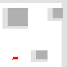
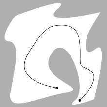
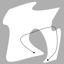
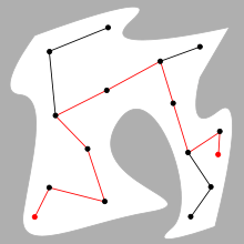
These approaches are similar to grid-based search approaches except that they generate a paving covering entirely the configuration space instead of a grid.^[1] The paving is decomposed into two subpavings X⁻,X⁺ made with boxes such that X⁻ ⊂ C_free ⊂ X⁺. Characterizing C_free amounts to solve a set inversion problem. Interval analysis could thus be used when C_free cannot be described by linear inequalities in order to have a guaranteed enclosure.

The robot is thus allowed to move freely in X⁻, and cannot go outside X⁺. To both subpavings, a neighbor graph is built and paths can be found using algorithms such as Dijkstra or A*. When a path is feasible in X⁻, it is also feasible in C_free. When no path exists in X⁺ from one initial configuration to the goal, we have the guarantee that no feasible path exists in C_free. As for the grid-based approach, the interval approach is inappropriate for high-dimensional problems, due to the fact that the number of boxes to be generated grows exponentially with respect to the dimension of configuration space.

An illustration is provided by the three figures on the right where a hook with two degrees of freedom has to move from the left to the right, avoiding two horizontal small segments.

Motion from the initial configuration (blue) to the final configuration of the hook, avoiding the two obstacles (red segments). The left-bottom corner of the hook has to stay on the horizontal line, which makes the hook two degrees of freedom.

Decomposition with boxes covering the configuration space: The subpaving X⁻ is the union all red boxes and the subpaving X⁺ is the union of red and green boxes. The path corresponds to the motion represented above.

This figure corresponds to the same path as above but obtained with many fewer boxes.The algorithm avoids bisecting boxes in parts of the configuration space that do not influence the final result.

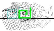
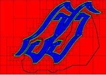
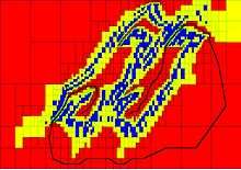
The decomposition with subpavings using interval analysis also makes it possible to characterize the topology of C_free such as counting its number of connected components.^[2]

Geometric algorithms

Point robots among polygonal obstacles

• Visibility graph
• Cell decomposition

Translating objects among obstacles

• Minkowski sum

Reward-based algorithms

Reward-based algorithms assume that the robot in each state (position and internal state, including direction) can choose between different actions (motion). However, the result of each action is not definite. In other words, outcomes (displacement) are partly random and partly under the control of the robot. The robot gets positive reward when it reaches the target and gets negative reward if it collides with an obstacle. These algorithms try to find a path which maximizes cumulative future rewards. The Markov decision process (MDP) is a popular mathematical framework that is used in many reward-based algorithms. The advantage of MDPs over other reward-based algorithms is that they generate the optimal path. The disadvantage of MDPs is that they limit the robot to choose from a finite set of actions. Therefore, the path is not smooth (similar to grid-based approaches).

Artificial potential fields

One approach is to treat the robot's configuration as a point in a potential field that combines attraction to the goal, and repulsion from obstacles. The resulting trajectory is output as the path. This approach has advantages in that the trajectory is produced with little computation. However, they can become trapped in local minima of the potential field and fail to find a path, or can find a non-optimal path. The artificial potential fields can be treated as continuum equations similar to electrostatic potential fields (treating the robot like a point charge), or motion through the field can be discretized using a set of linguistic rules.

Sampling-based algorithms

Sampling-based algorithms represent the configuration space with a roadmap of sampled configurations. A basic algorithm samples N configurations in C, and retains those in C_free to use as milestones. A roadmap is then constructed that connects two milestones P and Q if the line segment PQ is completely in C_free. Again, collision detection is used to test inclusion in C_free. To find a path that connects S and G, they are added to the roadmap. If a path in the roadmap links S and G, the planner succeeds, and returns that path. If not, the reason is not definitive: either there is no path in C_free, or the planner did not sample enough milestones.

These algorithms work well for high-dimensional configuration spaces, because unlike combinatorial algorithms, their running time is not (explicitly) exponentially dependent on the dimension of C. They are also (generally) substantially easier to implement. They are probabilistically complete, meaning the probability that they will produce a solution approaches 1 as more time is spent. However, they cannot determine if no solution exists.

Given basic visibility conditions on C_free, it has been proven that as the number of configurations N grows higher, the probability that the above algorithm finds a solution approaches 1 exponentially.^[3] Visibility is not explicitly dependent on the dimension of C; it is possible to have a high-dimensional space with "good" visibility or a low-dimensional space with "poor" visibility. The experimental success of sample-based methods suggests that most commonly seen spaces have good visibility.

There are many variants of this basic scheme:

• It is typically much faster to only test segments between nearby pairs of milestones, rather than all pairs.
• Nonuniform sampling distributions attempt to place more milestones in areas that improve the connectivity of the roadmap.
• Quasirandom samples typically produce a better covering of configuration space than pseudorandom ones, though some recent work argues that the effect of the source of randomness is minimal compared to the effect of the sampling distribution.
• It is possible to substantially reduce the number of milestones needed to solve a given problem by allowing curved eye sights (for example by crawling on the obstacles that block the way between two milestones ^[4]).
• If only one or a few planning queries are needed, it is not always necessary to construct a roadmap of the entire space. Tree-growing variants are typically faster for this case (single-query planning). Roadmaps are still useful if many queries are to be made on the same space (multi-query planning)

List of notable algorithms

• A*
• D*
• Rapidly-exploring random tree
• Probabilistic roadmap

Differential constraints

Holonomic

• Manipulator arms (with dynamics)

Nonholonomic

• Cars
• Unicycles
• Planes
• Acceleration bounded systems
• Moving obstacles (time cannot go backward)
• Bevel-tip steerable needle
• Differential Drive Robots

Hybrid systems

Hybrid systems are those that mix discrete and continuous behavior. Examples of such systems are:

• Robotic manipulation
• Mechanical assembly
• Legged robot locomotion
• Reconfigurable robots

Uncertainty

• Motion uncertainty
• Missing information
• Active sensing
• Sensorless planning

References

- ↑ Jaulin, L. (2001). "Path planning using intervals and graphs" (PDF). Reliable Computing. 7 (1).
- ↑ Delanoue, N.; Jaulin, L.; Cottenceau, B. (2006). "Counting the Number of Connected Components of a Set and Its Application to Robotics" (PDF). Applied Parallel Computing, Lecture Notes in Computer Science. 3732 (1).
- ↑ Hsu, D.; J.C. Latombe, J.C.; Motwani, R. (1997). "Path Planning in Expansive Configuration Spaces". Proc. IEEE Int. Conf. on Robotics and Automation.
- ↑ Shvalb, N.; Ben Moshe, B.; Medina, O. (2013). "A real-time motion planning algorithm for a hyper-redundant set of mechanisms". Robotica. 31 (8): 1327–1335. doi:10.1017/S0263574713000489.
Further reading
- Robot Motion Planning, Jean-Claude Latombe, 1991, Kluwer Academic Publishers
- Planning Algorithms, Steven M. LaValle, 2006, Cambridge University Press, ISBN 0-521-86205-1.
- Principles of Robot Motion: Theory, Algorithms, and Implementation, H. Choset, W. Burgard, S. Hutchinson, G. Kantor, L. E. Kavraki, K. Lynch, and S. Thrun, MIT Press, April 2005.
- Mark de Berg; Marc van Kreveld; Mark Overmars & Otfried Schwarzkopf (2000). Computational Geometry (2nd revised ed.). Springer-Verlag. ISBN 3-540-65620-0. Chapter 13: Robot Motion Planning: pp. 267–290.
External links