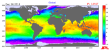
Regional Ocean Modeling System

Regional Ocean Modeling System (ROMS) is a free-surface, terrain-following, primitive equations ocean model widely used by the scientific community for a diverse range of applications. The model is developed and supported by researchers at the Rutgers University, University of California Los Angeles and contributors worldwide.
ROMS is primarily used to model how a given region of the ocean responds to physical forcings such as heating or wind. It can also be used to model how a given ocean system responds to inputs like sediment, freshwater, ice, or nutrients, requiring coupled models nested within the ROMS framework.
Framework
Central to the ROMS model are four models that form what is called the dynamical center or "kernel" of the model:
- Nonlinear kernel (NLM)[1][2]
- Tangent linear kernel (TLM)
- Representer tangent linear kernel (RPM)
- Adjoint kernel (ADM)[3]
ROMS is a 4D model, i.e. a 3-dimensional model that can be run to evaluate change over a given amount of time. It is gridded in vertical layers that make up the water column and horizontal cells that make up the coordinates of the 2D cartesian plane of the model region. The grid can be squeezed or stretched to increase or decrease the resolution for an area of interest, such as a thermocline. Grid stretching in the vertical direction follows bottom topography, allowing for the idealized flow of water over features such as seamounts.[4]
In both the vertical and horizontal directions, the default equations use centered, second-order finite difference schemes on staggered grids. Higher order schemes are available if desired, for example using parabolic spline reconstruction.[2]
Boundaries such as coastlines can be specified for a given region using land- and sea-masking. The top vertical boundary, the air-sea interface, uses an interaction scheme developed by Fairall et al. (1996).[5] The bottom vertical boundary, the sediment-water interface, uses a bottom stress or bottom-boundary-layer scheme developed by Styles and Glenn (2000).[6]
Source code and output
ROMS uses an open-access source code that can be downloaded by filling out an online request form. It runs on C-processing and was developed for shared computing uses. The model run must be initialized or compiled before it is run. The output format of model run files is netCDF. Model output is often visualized using independent secondary programming software such as MATLAB or Python.
Applications

The versatility of ROMS has been proven in its diverse applications to different systems and regions. It is best applied to mesoscale systems,[7] or those systems that can be mapped at high resolution, such as 1-km to 100-km grid spacing.
Coupled model applications
Biogeochemical, bio-optical, sea ice, sediment, and other models can be nested within the ROMS framework to study specific processes. These are usually developed for specific regions of the world's oceans but can be applied elsewhere. For example, the sea ice application of ROMS was originally developed for the Barents Sea Region.[8]
ROMS modeling efforts are increasingly being coupled with observational platforms, such as buoys, satellites, and ship-mounted underway sampling systems, to provide more accurate forecasting of ocean conditions.
Regional applications
There is an ever-growing number of applications of ROMS to particular regions of the world's oceans. These integrated ocean modeling systems use ROMS for the circulation component, and add other variables and processes of interest. A few examples are:
See also
References
- ↑ Shchepetkin, Alexander F. (2003). "A method for computing horizontal pressure-gradient force in an oceanic model with a nonaligned vertical coordinate". Journal of Geophysical Research. 108 (C3). doi:10.1029/2001jc001047. ISSN 0148-0227.
- 1 2 Shchepetkin, A.F.; McWilliams, J.C. (2005). The Regional Ocean Modeling System: A Split-Explicit, Free-Surface, Topography-Following-Coordinate Ocean Model, 2003. Los Angeles, California: University of California at Los Angeles: Institute of Geophysics and Planetary Physics.
- ↑ "A comprehensive ocean prediction and analysis system based on the tangent linear and adjoint of a regional ocean model". Ocean Modelling. 7 (1–2): 227–258. 2004-01-01. doi:10.1016/j.ocemod.2003.11.001. ISSN 1463-5003.
- ↑ "A Semi-implicit Ocean Circulation Model Using a Generalized Topography-Following Coordinate System". Journal of Computational Physics. 115 (1): 228–244. 1994-11-01. doi:10.1006/jcph.1994.1189. ISSN 0021-9991.
- ↑ Fairall, C. W.; Bradley, E. F.; Rogers, D. P.; Edson, J. B.; Young, G. S. (1996-02-15). "Bulk parameterization of air-sea fluxes for Tropical Ocean-Global Atmosphere Coupled-Ocean Atmosphere Response Experiment". Journal of Geophysical Research: Oceans. 101 (C2): 3747–3764. doi:10.1029/95jc03205. ISSN 0148-0227.
- ↑ Styles, Richard; Glenn, Scott M. (2000-10-15). "Modeling stratified wave and current bottom boundary layers on the continental shelf". Journal of Geophysical Research: Oceans. 105 (C10): 24119–24139. doi:10.1029/2000jc900115. ISSN 0148-0227.
- ↑ "Met Office: Mesoscale modelling". 2010-12-29. Retrieved 2018-04-26.
- ↑ Budgell, W. P. (2005-12-01). "Numerical simulation of ice-ocean variability in the Barents Sea region". Ocean Dynamics. 55 (3–4): 370–387. doi:10.1007/s10236-005-0008-3. ISSN 1616-7341.
- ↑ "Development of a Coupled Ocean–Atmosphere–Wave–Sediment Transport (COAWST) Modeling System". Ocean Modelling. 35 (3): 230–244. 2010-01-01. doi:10.1016/j.ocemod.2010.07.010. ISSN 1463-5003.
- ↑ Feng, Yang; Friedrichs, Marjorie A. M.; Wilkin, John; Tian, Hanqin; Yang, Qichun; Hofmann, Eileen E.; Wiggert, Jerry D.; Hood, Raleigh R. (2015). "Chesapeake Bay nitrogen fluxes derived from a land-estuarine ocean biogeochemical modeling system: Model description, evaluation, and nitrogen budgets". Journal of Geophysical Research: Biogeosciences. 120 (8): 1666–1695. doi:10.1002/2015jg002931. PMC 5014239. PMID 27668137.
- ↑ "Intrinsic and forced interannual variability of the Gulf of Alaska mesoscale circulation". Progress in Oceanography. 75 (2): 266–286. 2007-10-01. doi:10.1016/j.pocean.2007.08.011. ISSN 0079-6611.