Ratio distribution

A ratio distribution (or quotient distribution) is a probability distribution constructed as the distribution of the ratio of random variables having two other known distributions. Given two (usually independent) random variables X and Y, the distribution of the random variable Z that is formed as the ratio

Z=X/Y

is a ratio distribution. (See also Relationships among probability distributions.) The Cauchy distribution is an example of a ratio distribution. The random variable associated with this distribution comes about as the ratio of two Gaussian (normal) distributed variables with zero mean. Thus the Cauchy distribution is also called the normal ratio distribution. A number of researchers have considered more general ratio distributions.^[1]^[2]^[3]^[4]^[5]^[6]^[7]^[8]^[9] Two distributions often used in test-statistics, the t-distribution and the F-distribution, are also ratio distributions: The t-distributed random variable is the ratio of a Gaussian random variable divided by an independent chi-distributed random variable (i.e., the square root of a chi-squared distribution), while the F-distributed random variable is the ratio of two independent chi-squared distributed random variables.

Often the ratio distributions are heavy-tailed, and it may be difficult to work with such distributions and develop an associated statistical test. A method based on the median has been suggested as a "work-around".^[10]

Algebra of random variables

The ratio is one type of algebra for random variables: Related to the ratio distribution are the product distribution, sum distribution and difference distribution. More generally, one may talk of combinations of sums, differences, products and ratios. Many of these distributions are described in Melvin D. Springer's book from 1979 The Algebra of Random Variables.^[8]

The algebraic rules known with ordinary numbers do not apply for the algebra of random variables. For example, if a product is C = AB and a ratio is D=C/A it does not necessarily mean that the distributions of D and B are the same. Indeed, a peculiar effect is seen for the Cauchy distribution: The product and the ratio of two independent Cauchy distributions (with the same scale parameter and the location parameter set to zero) will give the same distribution.^[8] This becomes evident when regarding the Cauchy distribution as itself a ratio distribution of two Gaussian distributions: Consider two Cauchy random variables, $C_{1}$ and $C_{2}$ each constructed from two Gaussian distributions $C_{1}=G_{1}/G_{2}$ and $C_{2}=G_{3}/G_{4}$ then

{\frac {C_{1}}{C_{2}}}={\frac {{G_{1}}/{G_{2}}}{{G_{3}}/{G_{4}}}}={\frac {G_{1}G_{4}}{G_{2}G_{3}}}={\frac {G_{1}}{G_{2}}}\times {\frac {G_{4}}{G_{3}}}=C_{1}\times C_{3},

where $C_{3}=G_{4}/G_{3}$ . The first term is the ratio of two Cauchy distributions while the last term is the product of two such distributions.

Derivation

A way of deriving the ratio distribution of Z from the joint distribution of the two other random variables, X and Y, is by integration of the following form^[3]

p_{Z}(z)=\int _{{-\infty }}^{{+\infty }}|y|\,p_{{X,Y}}(zy,y)\,dy.

This is not always straightforward.

The Mellin transform has also been suggested for derivation of ratio distributions.^[8]

Moments of Random Ratios

From Mellin transform theory, for distributions existing only on the positive half-line $x\geq 0$ , we have the product identity $\mathbb {E} [(UV)^{p}]=\mathbb {E} [U^{p}]\;\mathbb {E} [V^{p}]$ provided $U,\;V$ are independent. For the case of a ratio of samples like $\mathbb {E} [(X/Y)^{p}]$ , in order to make use of this identity it is necessary to use moments of the inverse distribution. Set $1/Y=Z$ such that $\mathbb {E} [(XZ)^{p}]=\mathbb {E} [X^{p}]\;\mathbb {E} [Y^{-p}]$ . Thus, if the moments of $X^{p}{\text{ and }}Y^{-p}$ can be determined separately, then the moments of $X/Y$ can be found. The moments of $Y^{-p}$ are determined from the inverse pdf of $Y$ , often a tractable exercise. At simplest, $\mathbb {E} [Y^{-p}]=\int _{0}^{\infty }y^{-p}f_{y}(y)dy$ .

To illustrate, let $X$ be sampled from a standard Gamma distribution $x^{\alpha -1}e^{-x}/\Gamma (\alpha ){\text{ whose }}p^{th}$ moment is $\Gamma (\alpha +p)/\Gamma (\alpha )$ .

$Z=Y^{-1}$ is sampled from an inverse Gamma distribution with parameter $\beta$ and has pdf $z^{1+\beta }e^{-1/z}/\Gamma (\beta )$ . The moments of this pdf are $\mathbb {E} [Z^{p}]=\mathbb {E} [Y^{-p}]={\frac {\Gamma (\beta -p)}{\Gamma (\beta )}},\;p<\beta$ .

Multiplying the corresponding moments gives $\mathbb {E} [(X/Y)^{p}]=\mathbb {E} [X^{p}]\;\mathbb {E} [Y^{-p}]={\frac {\Gamma (\alpha +p)}{\Gamma (\alpha )}}{\frac {\Gamma (\beta -p)}{\Gamma (\beta )}},\;p<\beta$ .

Independently, it is known that the ratio of the two Gamma samples $R=X/Y$ follows the Beta Prime distribution: $f^{\beta ^{'}}(r,\alpha ,\beta )=B(\alpha ,\beta )^{-1}r^{\alpha -1}(1+r)^{-(\alpha +\beta )}$ whose moments are $\mathbb {E} [R^{p}]={\frac {\mathrm {B} (\alpha +p,\beta -p)}{\mathrm {B} (\alpha ,\beta )}}$

Substituting $\mathrm {B} (\alpha ,\beta )={\frac {\Gamma (\alpha )\Gamma (\beta )}{\Gamma (\alpha +\beta )}}$ we have $\mathbb {E} [R^{p}]={\frac {\Gamma (\alpha +p)\Gamma (\beta -p)}{\Gamma (\alpha +\beta )}}{\Bigg /}{\frac {\Gamma (\alpha )\Gamma (\beta )}{\Gamma (\alpha +\beta )}}={\frac {\Gamma (\alpha +p)\Gamma (\beta -p)}{\Gamma (\alpha )\Gamma (\beta )}}$ which is consistent with the product of moments above.

Gaussian ratio distribution

When X and Y are independent and have a Gaussian distribution with zero mean, the form of their ratio distribution is fairly simple: It is a Cauchy distribution. However, when the two distributions have non-zero means then the form for the distribution of the ratio is much more complicated. In 1932 Fieller^[2] removed all approximation from Geary's earlier result but his algorithm, as published, is not quite computer-ready due to the Gaussian integral in the final result (eqns 23-24) possibly going backward along the axis which needs to be trapped out. Here it is given in the more succinct form presented by David Hinkley.^[6] In the absence of correlation (cor(X,Y) = 0), the probability density function of the two normal variable X = N(μ_X, σ_X²) and Y = N(μ_Y, σ_Y²) ratio Z = X/Y is given by the following expression:

p_{Z}(z)={\frac {b(z)\cdot d(z)}{a^{3}(z)}}{\frac {1}{{\sqrt {2\pi }}\sigma _{x}\sigma _{y}}}\left[\Phi \left({\frac {b(z)}{a(z)}}\right)-\Phi \left(-{\frac {b(z)}{a(z)}}\right)\right]+{\frac {1}{a^{2}(z)\cdot \pi \sigma _{x}\sigma _{y}}}e^{{-{\frac {c}{2}}}}

where

a(z)={\sqrt {{\frac {1}{\sigma _{x}^{2}}}z^{2}+{\frac {1}{\sigma _{y}^{2}}}}}

b(z)={\frac {\mu _{x}}{\sigma _{x}^{2}}}z+{\frac {\mu _{y}}{\sigma _{y}^{2}}}

c={\frac {\mu _{x}^{2}}{\sigma _{x}^{2}}}+{\frac {\mu _{y}^{2}}{\sigma _{y}^{2}}}

d(z)=e^{{{\frac {b^{2}(z)-ca^{2}(z)}{2a^{2}(z)}}}}

And $\Phi$ is the cumulative distribution function of the Normal distribution

\Phi (t)=\int _{{-\infty }}^{{t}}\,{\frac {1}{{\sqrt {2\pi }}}}e^{{-{\frac {1}{2}}u^{2}}}\ du\

The above expression becomes even more complicated if the variables X and Y are correlated. In the case that $\mu _{x}=\mu _{y}=0$ and $\sigma _{x}=\sigma _{y}=1$ we have the standard Cauchy distribution. This is most easily derived by a change of variable. Since $\theta =\arctan({\frac {Y}{X}})$ is uniformly distributed on $[-\pi /2,\pi /2]$ for the bivariate Normal distribution then in the right hand semicircle we have $p(\theta )=1/\pi$ . Defining $t=\tan(\theta )={\frac {Y}{X}}$ we have $p_{\theta }(t)=p(\theta )/|dt/d\theta |=\sec ^{2}(\theta )/\pi$ . Finally set $\sec ^{2}(\theta )=1/(1+t^{2})$ to get $p_{t}(t)={\frac {1}{\pi (1+t^{2})}}$ and by circular symmetry, $p(z)=p(X/Y)={\frac {1}{\pi (1+z^{2})}}$ .

If $\sigma _{X}\neq 1$ , $\sigma _{Y}\neq 1$ or $\rho \neq 0$ the more general Cauchy distribution is obtained

p_{Z}(z)={\frac {1}{\pi }}{\frac {\beta }{(z-\alpha )^{2}+\beta ^{2}}},

where ρ is the correlation coefficient between X and Y and

\alpha =\rho {\frac {\sigma _{x}}{\sigma _{y}}},

\beta ={\frac {\sigma _{x}}{\sigma _{y}}}{\sqrt {1-\rho ^{2}}}.

The complex distribution has also been expressed with Kummer's confluent hypergeometric function or the Hermite function.^[9]

A transformation to Gaussianity

A transformation has been suggested so that, under certain assumptions, the transformed variable T would approximately have a standard Gaussian distribution:^[1]

t\approx {\frac {\mu _{y}z-\mu _{x}}{\sqrt {\sigma _{y}^{2}z^{2}-2\rho \sigma _{x}\sigma _{y}z+\sigma _{x}^{2}}}}

The transformation has been called the Geary–Hinkley transformation,^[7] and the approximation is good if Y is unlikely to assume negative values.

Correlated normal ratio

Geary showed how the correlated ratio $z$ could be transformed into a near-Gaussian form and developed an approximation for $t$ dependent on the probability of negative denominator values $x+\mu _{x}<0$ being vanishingly small. Fieller's later correlated ratio analysis is exact but cumbersome and incompatible with modern math packages without manual intervention to ensure the Normal integral always is defined in a positive direction. The latter problem can also be identified in some of Marsaglia's equations. Hinkley's correlated results are exact but it is shown below that the correlated ratio condition can be transformed simply into an uncorrelated one so only the simplified Hinkley equations above are required, not the full correlated ratio version.

Let the ratio be $z={\frac {x+\mu _{x}}{y+\mu _{y}}}$ in which $x,y$ are zero-mean correlated normal variables with variances $\sigma _{x}^{2},\sigma _{y}^{2}$ and $X,Y$ have means $\mu _{x},\mu _{y}$ .
We can in general write $x'=x-\rho y\sigma _{x}/\sigma _{y}$ such that $x',y$ become uncorrelated and $x'$ has standard deviation $\sigma _{x}'=\sigma _{x}{\sqrt {1-\rho ^{2}}}$ .
The ratio $z={\frac {x'+\rho y\sigma _{x}/\sigma _{y}+\mu _{x}}{y+\mu _{y}}}$ is invariant and retains the same pdf.

The $y$ term in the numerator is made separable by expanding
${x'+\rho y\sigma _{x}/\sigma _{y}+\mu _{x}}=x'+\mu _{x}-\rho \mu _{y}{\frac {\sigma _{x}}{\sigma _{y}}}+\rho (y+\mu _{y}){\frac {\sigma _{x}}{\sigma _{y}}}$
to get
$z={\frac {x'+\mu _{x}'}{y+\mu _{y}}}+\rho {\frac {\sigma _{x}}{\sigma _{y}}}$
in which
$\mu '_{x}=\mu _{x}-\rho \mu _{y}{\frac {\sigma _{x}}{\sigma _{y}}}$ .

Finally, to be explicit, the pdf of the ratio $z$ for correlated variables is found by inputting the modified parameters $\sigma _{x}',\mu _{x}',\sigma _{y},\mu _{y}$ and $\rho '=0$ into the Hinkley equation above which returns the pdf for the correlated ratio with an offset $-\rho {\frac {\sigma _{x}}{\sigma _{y}}}$ on $z$ . In retrospect this transformation will be recognized as being the same as that used by Geary as a partial result in his eqn viii but which is not well-explained and shows that part of Geary's transformation is not dependent on the positivity of Y

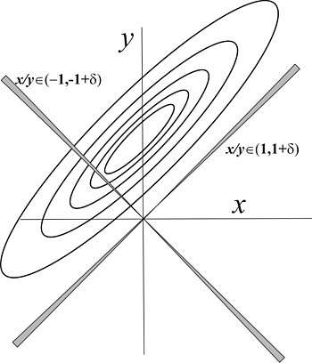
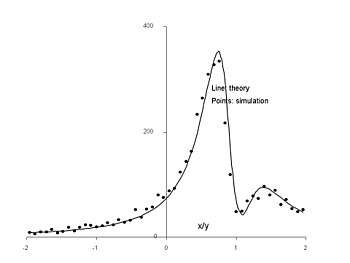
The figures below show an example of a positively correlated ratio with $\sigma _{x}=\sigma _{y}=1,\mu _{x}=0,\mu _{y}=0.5,\rho =0.975$ in which the shaded areas represent the increment of area selected by given ratio $x/y\in [r,r+\delta ]$ which accumulates probability from the distribution. The theoretical distribution below, derived from the equations under discussion combined with Hinkley's equations, is highly consistent with a simulation result using 5,000 samples. In the top figure it is easily understood that for a ratio $z=x/y=1$ the line almost bypasses the distribution mass altogether and this coincides with a near-zero region in the theoretical pdf. Conversely as $x/y$ reduces toward zero the line collects a higher probability.

Contours of the bivariate Gaussian distribution (not to scale)

pdf of the ratio z and a simulation (points) for

\sigma _{x}=\sigma _{y}=1,\mu _{x}=0,\mu _{y}=0.5,\rho =0.975

Example of a correlated normal ratio

Uniform ratio distribution

With two independent random variables following a uniform distribution, e.g.,

p_{X}(x)={\begin{cases}1\qquad 0<x<1\\0\qquad {\mbox{otherwise}}\end{cases}}

the ratio distribution becomes

p_{Z}(z)={\begin{cases}1/2\qquad &0<z<1\\{\frac {1}{2z^{2}}}\qquad &z\geq 1\\0\qquad &{\mbox{otherwise}}\end{cases}}

Cauchy ratio distribution

If two independent random variables, X and Y each follow a Cauchy distribution with median equal to zero and shape factor $a$

p_{X}(x|a)={\frac {a}{\pi (a^{2}+x^{2})}}

then the ratio distribution for the random variable $Z=X/Y$ is ^[11]

p_{Z}(z|a)={\frac {1}{\pi ^{2}(z^{2}-1)}}\ln \left(z^{2}\right).

This distribution does not depend on $a$ and the result stated by Springer ^[8] (p158 Question 4.6) is not correct. The ratio distribution is similar to but not the same as the product distribution of the random variable $W=XY$ :

p_{W}(w|a)={\frac {a^{2}}{\pi ^{2}(w^{2}-a^{4})}}\ln \left({\frac {w^{2}}{a^{4}}}\right).

^[8]

More generally, if two independent random variables X and Y each follow a Cauchy distribution with median equal to zero and shape factor $a$ and $b$ respectively, then:

1. The ratio distribution for the random variable $Z=X/Y$ is ^[11]

p_{Z}(z|a,b)={\frac {ab}{\pi ^{2}(b^{2}z^{2}-a^{2})}}\ln \left({\frac {b^{2}z^{2}}{a^{2}}}\right).

2. The product distribution for the random variable $W=XY$ is ^[11]

p_{W}(w|a,b)={\frac {ab}{\pi ^{2}(w^{2}-a^{2}b^{2})}}\ln \left({\frac {w^{2}}{a^{2}b^{2}}}\right).

The result for the ratio distribution can be obtained from the product distribution by replacing $b$ with ${\frac {1}{b}}.$

Ratio of standard normal to standard uniform

If X has a standard normal distribution and Y has a standard uniform distribution, then Z = X / Y has a distribution known as the slash distribution, with probability density function

p_{Z}(z)={\begin{cases}\left[\phi (0)-\phi (z)\right]/z^{2}\quad &z\neq 0\\\phi (0)/2\quad &z=0,\\\end{cases}}

where φ(z) is the probability density function of the standard normal distribution.^[12]

Other ratio distributions

Let X be a normal(0,1) distribution, Y and Z be chi square distributions with m and n degrees of freedom respectively, all independent, with $f^{\chi }(x,k)={\frac {x^{{\frac {k}{2}}-1}e^{-x/2}}{2^{k/2}\Gamma (k/2)}}$ . Then

{\frac {X}{{\sqrt {Y/m}}}}=t_{m}

{\frac {Y/m}{Z/n}}=F_{{m,n}}

{\frac {Y}{Y+Z}}=\beta (m/2,n/2)

If U is gamma ( α₁, 1) and V is gamma (α₂, 1) distributed, where $\Gamma (x,\alpha ,1)={\frac {x^{\alpha -1}e^{-x}}{\Gamma (\alpha )}}$ , then

{\frac {U}{U+V}}\sim \beta (\alpha _{1},\alpha _{2})

{\frac {U}{V}}\sim \beta '(\alpha _{1},\alpha _{2})

{\frac {V}{U}}\sim \beta '(\alpha _{2},\alpha _{1})

where t_m is Student's t distribution, $F$ is the F distribution, $\beta$ is the beta distribution, $\beta '$ is the beta prime distribution and $\Gamma$ is the gamma distribution

Scaling: if U is a sample from $\Gamma (x,\alpha ,1)$ then $\theta$ U is a sample from $\Gamma (x,\alpha ,\theta )$ where $\Gamma (x,\alpha ,\theta )={\frac {x^{\alpha -1}e^{-{\frac {x}{\theta }}}}{\theta ^{k}\Gamma (\alpha )}}$

thus, if U is

\Gamma (\alpha _{1},\theta _{1})

and V is

\Gamma (\alpha _{2},\theta _{2})

distributed, then by rescaling the

\theta

parameter to unity we have, trivially

{\frac {\frac {U}{\theta _{1}}}{{\frac {U}{\theta _{1}}}+{\frac {V}{\theta _{2}}}}}={\frac {\theta _{2}U}{\theta _{2}U+\theta _{1}V}}\sim \beta (\alpha _{1},\alpha _{2})

{\frac {\frac {U}{\theta _{1}}}{\frac {V}{\theta _{2}}}}={\frac {\theta _{2}}{\theta _{1}}}{\frac {U}{V}}\sim \beta '(\alpha _{1},\alpha _{2})

thus

{\frac {U}{V}}\sim \beta '(\alpha _{1},\alpha _{2},1,{\frac {\theta _{1}}{\theta _{2}}})

where

\beta '(\alpha _{1},\alpha _{2},p,q)

is the generalized Beta prime distribution

i.e. if

X\sim \beta '(\alpha _{1},\alpha _{2},1,1)

then

\theta X\sim \beta '(\alpha _{1},\alpha _{2},1,\theta )

Other Gamma Distributions

Generalized gamma distribution

The Gamma distribution can be generalized to

$f(x,a,d,p)={\frac {p}{\Gamma (d/p)a^{d}}}x^{d-1}e^{-(x/a)^{p}}\;x\geq 0;a,\;d,\;p>0$
which includes the regular gamma, chi, chi-squared, exponential and Weibull distributions.

If

U\sim f(x,a_{1},d_{1},p),\;\;V\sim f(x,a_{2},d_{2},p){\text{ are independent, and  }}W=U/V

then ^[13]

$g(w)={\frac {p\left({\frac {a_{1}}{a_{2}}}\right)^{d_{2}}}{B\left({\frac {d_{1}}{p}},{\frac {d_{2}}{p}}\right)}}{\frac {w^{-d_{2}-1}}{\left(1+\left({\frac {a_{2}}{a_{1}}}\right)^{-p}w^{-p}\right)^{\frac {d_{1}+d_{2}}{p}}}},\;\;w>0$

Modelling a mixture of different scaling factors

In the ratios above, Gamma samples, U, V may have differing sample sizes $\alpha _{1},\alpha _{2}$ but must be drawn from the same distribution ${\frac {x^{\alpha -1}e^{-{\frac {x}{\theta }}}}{\theta ^{k}\Gamma (\alpha )}}$ with equal scaling $\theta$ .
In situations where U and V are differently scaled, a variables transformation allows the modified random ratio pdf to be determined. Let $X={\frac {U}{U+V}}={\frac {1}{1+B}}$ where $U\sim \Gamma (\alpha _{1},\theta ),V\sim \Gamma (\alpha _{2},\theta ),\theta$ arbitrary
and, from above, $X\sim Beta(\alpha _{1},\alpha _{2}),B=V/U\sim Beta'(\alpha _{2},\alpha _{1})$ .
Rescale V arbitrarily, defining $Y\sim {\frac {U}{U+\phi V}}={\frac {1}{1+\phi B}},\;\;0\leq \phi \leq \infty$

We have $B={\frac {1-X}{X}}$ and substitution into Y gives $Y={\frac {X}{\phi +(1-\phi )X}},dY/dX={\frac {\phi }{(\phi +(1-\phi )X)^{2}}}$
Transforming X to Y gives $f_{Y}(Y)={\frac {f_{X}(X)}{|dY/dX|}}={\frac {\beta (X,\alpha _{1},\alpha _{2})}{\phi /[\phi +(1-\phi )X]^{2}}}$
Noting $X={\frac {\phi Y}{1-(1-\phi )Y}}$ we finally have

f_{Y}(Y,\phi )={\frac {\phi }{[1-(1-\phi )Y]^{2}}}\beta \left({\frac {\phi Y}{1-(1-\phi )Y}},\alpha _{1},\alpha _{2}\right),\;\;\;0\leq Y\leq 1

Thus, if $U\sim \Gamma (\alpha _{1},\theta _{1})$ and $V\sim \Gamma (\alpha _{2},\theta _{2})$
then $Y={\frac {U}{U+V}}$ is distributed as $f_{Y}(Y,\phi )$ with $\phi ={\frac {\theta _{2}}{\theta _{1}}}$

The distribution of Y is limited here to the interval [0,1]. It can be generalized by scaling such that if $Y\sim f_{Y}(Y,\phi )$ then

\Theta Y\sim f_{Y}(Y,\phi ,\Theta )

where $f_{Y}(Y,\phi ,\Theta )={\frac {\phi /\Theta }{[1-(1-\phi )Y/\Theta ]^{2}}}\beta \left({\frac {\phi Y/\Theta }{1-(1-\phi )Y/\Theta }},\alpha _{1},\alpha _{2}\right),\;\;\;0\leq Y\leq \Theta$

\Theta Y

is then a sample from

{\frac {\Theta U}{U+\phi V}}

Though not ratio distributions of two variables, the following identities are useful:

If

X\sim \beta (\alpha ,\beta )

then

{\frac {X}{1-X}}\sim \beta '(\alpha ,\beta )

If

Y\sim \beta '(\alpha ,\beta )

then

{\frac {1}{Y}}\sim \beta '(\beta ,\alpha )

If

Y\sim \beta '(\alpha ,\beta )

then

{\frac {Y}{1+Y}}\sim \beta (\alpha ,\beta )

If

Y\sim \beta '(\alpha ,\beta )

then

{\frac {1}{1+Y}}\sim \beta (\beta ,\alpha )

thus, from above,

{\frac {U/V}{1+U/V}}={\frac {U}{V+U}}\sim \beta (\alpha ,\beta )

If X and Y are exponential random variables with mean μ, then X-Y is a double exponential random variable with mean 0 and scale μ.

Binomial distribution

This result was first derived by Katz et al in 1978.^[14]

Let p₁ and p₂ be the probabilities of success in the binomial distributions B(X,n) and B(Y,m) respectively. Let T = (X/n)/(Y/m).

Then log(T) is approximately normally distributed with mean log(p₁/p₂) and variance (1/x) - (1/n) + (1/y) - (1/m).

Ratio distributions in multivariate analysis

Ratio distributions also appear in multivariate analysis. If the random matrices X and Y follow a Wishart distribution then the ratio of the determinants

\phi =|{\mathbf {X}}|/|{\mathbf {Y}}|

is proportional to the product of independent F random variables. In the case where X and Y are from independent standardized Wishart distributions then the ratio

\Lambda ={|{\mathbf {X}}|/|{\mathbf {X}}+{\mathbf {Y}}|}

has a Wilks' lambda distribution.

References

1 2 Geary, R. C. (1930). "The Frequency Distribution of the Quotient of Two Normal Variates". Journal of the Royal Statistical Society. 93 (3): 442–446. doi:10.2307/2342070. JSTOR 2342070.
1 2 Fieller, E. C. (November 1932). "The Distribution of the Index in a Normal Bivariate Population". Biometrika. 24 (3/4): 428–440. doi:10.2307/2331976. JSTOR 2331976.
1 2 Curtiss, J. H. (December 1941). "On the Distribution of the Quotient of Two Chance Variables". The Annals of Mathematical Statistics. 12 (4): 409–421. doi:10.1214/aoms/1177731679. JSTOR 2235953.
↑ George Marsaglia (April 1964). Ratios of Normal Variables and Ratios of Sums of Uniform Variables. Defense Technical Information Center.
↑ Marsaglia, George (March 1965). "Ratios of Normal Variables and Ratios of Sums of Uniform Variables". Journal of the American Statistical Association. 60 (309): 193–204. doi:10.2307/2283145. JSTOR 2283145.
1 2 Hinkley, D. V. (December 1969). "On the Ratio of Two Correlated Normal Random Variables". Biometrika. 56 (3): 635–639. doi:10.2307/2334671. JSTOR 2334671.
1 2 Hayya, Jack; Armstrong, Donald; Gressis, Nicolas (July 1975). "A Note on the Ratio of Two Normally Distributed Variables". Management Science. 21 (11): 1338–1341. doi:10.1287/mnsc.21.11.1338. JSTOR 2629897.
1 2 3 4 5 6 Springer, Melvin Dale (1979). The Algebra of Random Variables. Wiley. ISBN 0-471-01406-0.
1 2 Pham-Gia, T.; Turkkan, N.; Marchand, E. (2006). "Density of the Ratio of Two Normal Random Variables and Applications". Communications in Statistics - Theory and Methods. Taylor & Francis. 35 (9): 1569–1591. doi:10.1080/03610920600683689.
↑ Brody, James P.; Williams, Brian A.; Wold, Barbara J.; Quake, Stephen R. (October 2002). "Significance and statistical errors in the analysis of DNA microarray data". Proc Natl Acad Sci U S A. 99 (20): 12975–12978. doi:10.1073/pnas.162468199. PMC 130571. PMID 12235357.
1 2 3 Kermond, John (2010). "An Introduction to the Algebra of Random Variables". Mathematical Association of Victoria 47th Annual Conference Proceedings - New Curriculum. New Opportunities. The Mathematical Association of Victoria: 1–16. ISBN 978-1-876949-50-1.
↑ "SLAPPF". Statistical Engineering Division, National Institute of Science and Technology. Retrieved 2009-07-02.
↑ B. Raja Rao, M. L. Garg. "A note on the generalized (positive) Cauchy distribution." "Canadian Mathematical Bulletin." 12(1969), 865-868 Published:1969-01-01
↑ Katz D. et al.(1978) Obtaining confidence intervals for the risk ratio in cohort studies. Biometrics 34:469–474

External links

This article is issued from Wikipedia. The text is licensed under Creative Commons - Attribution - Sharealike. Additional terms may apply for the media files.

[GearyR1930Frequency-1] 1 2 Geary, R. C. (1930). "The Frequency Distribution of the Quotient of Two Normal Variates". Journal of the Royal Statistical Society. 93 (3): 442–446. doi:10.2307/2342070. JSTOR 2342070.

[Fieller1932On-2] 1 2 Fieller, E. C. (November 1932). "The Distribution of the Index in a Normal Bivariate Population". Biometrika. 24 (3/4): 428–440. doi:10.2307/2331976. JSTOR 2331976.

[CurtissJ1941On-3] 1 2 Curtiss, J. H. (December 1941). "On the Distribution of the Quotient of Two Chance Variables". The Annals of Mathematical Statistics. 12 (4): 409–421. doi:10.1214/aoms/1177731679. JSTOR 2235953.

[4] George Marsaglia (April 1964). Ratios of Normal Variables and Ratios of Sums of Uniform Variables. Defense Technical Information Center.

[5] Marsaglia, George (March 1965). "Ratios of Normal Variables and Ratios of Sums of Uniform Variables". Journal of the American Statistical Association. 60 (309): 193–204. doi:10.2307/2283145. JSTOR 2283145.

[HinkleyD1969On-6] 1 2 Hinkley, D. V. (December 1969). "On the Ratio of Two Correlated Normal Random Variables". Biometrika. 56 (3): 635–639. doi:10.2307/2334671. JSTOR 2334671.

[HayyaJ1975On-7] 1 2 Hayya, Jack; Armstrong, Donald; Gressis, Nicolas (July 1975). "A Note on the Ratio of Two Normally Distributed Variables". Management Science. 21 (11): 1338–1341. doi:10.1287/mnsc.21.11.1338. JSTOR 2629897.

[SpringerM1979Algebra-8] 1 2 3 4 5 6 Springer, Melvin Dale (1979). The Algebra of Random Variables. Wiley. ISBN 0-471-01406-0.

[PhamGiaT2006Density-9] 1 2 Pham-Gia, T.; Turkkan, N.; Marchand, E. (2006). "Density of the Ratio of Two Normal Random Variables and Applications". Communications in Statistics - Theory and Methods. Taylor & Francis. 35 (9): 1569–1591. doi:10.1080/03610920600683689.

[10] Brody, James P.; Williams, Brian A.; Wold, Barbara J.; Quake, Stephen R. (October 2002). "Significance and statistical errors in the analysis of DNA microarray data". Proc Natl Acad Sci U S A. 99 (20): 12975–12978. doi:10.1073/pnas.162468199. PMC 130571. PMID 12235357.

[Kermond2010-11] 1 2 3 Kermond, John (2010). "An Introduction to the Algebra of Random Variables". Mathematical Association of Victoria 47th Annual Conference Proceedings - New Curriculum. New Opportunities. The Mathematical Association of Victoria: 1–16. ISBN 978-1-876949-50-1.

[nist-12] "SLAPPF". Statistical Engineering Division, National Institute of Science and Technology. Retrieved 2009-07-02.

[13] B. Raja Rao, M. L. Garg. "A note on the generalized (positive) Cauchy distribution." "Canadian Mathematical Bulletin." 12(1969), 865-868 Published:1969-01-01

[Katz1978-14] Katz D. et al.(1978) Obtaining confidence intervals for the risk ratio in cohort studies. Biometrics 34:469–474