Newton's method

In numerical analysis, Newton's method (also known as the Newton–Raphson method), named after Isaac Newton and Joseph Raphson, is a method for finding successively better approximations to the roots (or zeroes) of a real-valued function. It is one example of a root-finding algorithm.

x:f(x)=0\,.

The Newton–Raphson method in one variable is implemented as follows:

The method starts with a function $f$ defined over the real numbers $x$ , the function's derivative $f'$ , and an initial guess $x 0$ for a root of the function $f$ . If the function satisfies the assumptions made in the derivation of the formula and the initial guess is close, then a better approximation $x 1$ is

x_{1}=x_{0}-{\frac {f(x_{0})}{f'(x_{0})}}\,.

Geometrically, $(x 1, 0)$ is the intersection of the $x$ -axis and the tangent of the graph of $f$ at $(x 0, f (x 0))$ .

The process is repeated as

x_{n+1}=x_{n}-{\frac {f(x_{n})}{f'(x_{n})}}\,

until a sufficiently accurate value is reached.

This algorithm is first in the class of Householder's methods, succeeded by Halley's method. The method can also be extended to complex functions and to systems of equations.

Description

The function

f

is shown in blue and the tangent line is in red. We see that

x n + 1

is a better approximation than

x n

for the root

x

of the function

f

.

The idea of the method is as follows: one starts with an initial guess which is reasonably close to the true root, then the function is approximated by its tangent line (which can be computed using the tools of calculus), and one computes the $x$ -intercept of this tangent line (which is easily done with elementary algebra). This $x$ -intercept will typically be a better approximation to the function's root than the original guess, and the method can be iterated.

Suppose $f : (a, b) \to ℝ$ is a differentiable function defined on the interval $(a, b)$ with values in the real numbers $ℝ$ . The formula for converging on the root can be easily derived. Suppose we have some current approximation $x n$ . Then we can derive the formula for a better approximation, $x n + 1$ by referring to the diagram on the right. The equation of the tangent line to the curve $y = f (x)$ at the point $x = x n$ is

y=f'(x_{n})\,(x-x_{n})+f(x_{n}),

where $f'$ denotes the derivative of the function $f$ .

The $x$ -intercept of this line (the value of $x$ such that $y = 0$ ) is then used as the next approximation to the root, $x n + 1$ . In other words, setting $y$ to zero and $x$ to $x n + 1$ gives

0=f'(x_{n})\,(x_{n+1}-x_{n})+f(x_{n}).

Solving for $x n + 1$ gives

x_{n+1}=x_{n}-{\frac {f(x_{n})}{f'(x_{n})}}.

We start the process off with some arbitrary initial value $x 0$ . (The closer to the zero, the better. But, in the absence of any intuition about where the zero might lie, a "guess and check" method might narrow the possibilities to a reasonably small interval by appealing to the intermediate value theorem.) The method will usually converge, provided this initial guess is close enough to the unknown zero, and that $f' (x 0) \neq 0$ . Furthermore, for a zero of multiplicity 1, the convergence is at least quadratic (see rate of convergence) in a neighbourhood of the zero, which intuitively means that the number of correct digits roughly at least doubles in every step. More details can be found in the analysis section below.

The Householder's methods are similar but have higher order for even faster convergence. However, the extra computations required for each step can slow down the overall performance relative to Newton's method, particularly if $f$ or its derivatives are computationally expensive to evaluate.

History

The name "Newton's method" is derived from Isaac Newton's description of a special case of the method in De analysi per aequationes numero terminorum infinitas (written in 1669, published in 1711 by William Jones) and in De metodis fluxionum et serierum infinitarum (written in 1671, translated and published as Method of Fluxions in 1736 by John Colson). However, his method differs substantially from the modern method given above: Newton applies the method only to polynomials. He does not compute the successive approximations $x n$ , but computes a sequence of polynomials, and only at the end arrives at an approximation for the root $x$ . Finally, Newton views the method as purely algebraic and makes no mention of the connection with calculus. Newton may have derived his method from a similar but less precise method by Vieta. The essence of Vieta's method can be found in the work of the Persian mathematician Sharaf al-Din al-Tusi, while his successor Jamshīd al-Kāshī used a form of Newton's method to solve $x P - N = 0$ to find roots of $N$ (Ypma 1995). A special case of Newton's method for calculating square roots was known much earlier and is often called the Babylonian method.

Newton's method was used by 17th-century Japanese mathematician Seki Kōwa to solve single-variable equations, though the connection with calculus was missing.

Newton's method was first published in 1685 in A Treatise of Algebra both Historical and Practical by John Wallis.^[1] In 1690, Joseph Raphson published a simplified description in Analysis aequationum universalis.^[2] Raphson again viewed Newton's method purely as an algebraic method and restricted its use to polynomials, but he describes the method in terms of the successive approximations $x n$ instead of the more complicated sequence of polynomials used by Newton. Finally, in 1740, Thomas Simpson described Newton's method as an iterative method for solving general nonlinear equations using calculus, essentially giving the description above. In the same publication, Simpson also gives the generalization to systems of two equations and notes that Newton's method can be used for solving optimization problems by setting the gradient to zero.

Arthur Cayley in 1879 in The Newton-Fourier imaginary problem was the first to notice the difficulties in generalizing Newton's method to complex roots of polynomials with degree greater than 2 and complex initial values. This opened the way to the study of the theory of iterations of rational functions.

Practical considerations

Newton's method is an extremely powerful technique—in general the convergence is quadratic: as the method converges on the root, the difference between the root and the approximation is squared (the number of accurate digits roughly doubles) at each step. However, there are some difficulties with the method.

Difficulty in calculating derivative of a function

Newton's method requires that the derivative be calculated directly. An analytical expression for the derivative may not be easily obtainable and could be expensive to evaluate. In these situations, it may be appropriate to approximate the derivative by using the slope of a line through two nearby points on the function. Using this approximation would result in something like the secant method whose convergence is slower than that of Newton's method.

Failure of the method to converge to the root

It is important to review the proof of quadratic convergence of Newton's Method before implementing it. Specifically, one should review the assumptions made in the proof. For situations where the method fails to converge, it is because the assumptions made in this proof are not met.

Overshoot

If the first derivative is not well behaved in the neighborhood of a particular root, the method may overshoot, and diverge from that root. An example of a function with one root, for which the derivative is not well behaved in the neighborhood of the root, is

f(x)=|x|^{a},\quad 0<a<{\tfrac {1}{2}}

for which the root will be overshot and the sequence of $x$ will diverge. For $a = 1 / 2$ , the root will still be overshot, but the sequence will oscillate between two values. For $1 / 2 < a < 1$ , the root will still be overshot but the sequence will converge, and for $a \geq 1$ the root will not be overshot at all.

In some cases, Newton's method can be stabilized by using successive over-relaxation, or the speed of convergence can be increased by using the same method.

Stationary point

If a stationary point of the function is encountered, the derivative is zero and the method will terminate due to division by zero.

Poor initial estimate

A large error in the initial estimate can contribute to non-convergence of the algorithm. To overcome this problem one can often linearise the function that is being optimized using calculus, logs, differentials, or even using evolutionary algorithms, such as the stochastic funnel algorithm. Good initial estimates lie close to the final globally optimal parameter estimate. In nonlinear regression, the sum of squared errors (SSE) is only "close to" parabolic in the region of the final parameter estimates. Initial estimates found here will allow the Newton–Raphson method to quickly converge. It is only here that the Hessian matrix of the SSE is positive and the first derivative of the SSE is close to zero.

Mitigation of non-convergence

In a robust implementation of Newton's method, it is common to place limits on the number of iterations, bound the solution to an interval known to contain the root, and combine the method with a more robust root finding method.

Slow convergence for roots of multiplicity greater than 1

If the root being sought has multiplicity greater than one, the convergence rate is merely linear (errors reduced by a constant factor at each step) unless special steps are taken. When there are two or more roots that are close together then it may take many iterations before the iterates get close enough to one of them for the quadratic convergence to be apparent. However, if the multiplicity $m$ of the root is known, the following modified algorithm preserves the quadratic convergence rate:^[3]

x_{n+1}=x_{n}-m{\frac {f(x_{n})}{f'(x_{n})}}.

This is equivalent to using successive over-relaxation. On the other hand, if the multiplicity $m$ of the root is not known, it is possible to estimate $m$ after carrying out one or two iterations, and then use that value to increase the rate of convergence.

Analysis

Suppose that the function $f$ has a zero at $α$ , i.e., $f (α) = 0$ , and $f$ is differentiable in a neighborhood of $α$ .

If $f$ is continuously differentiable and its derivative is nonzero at $α$ , then there exists a neighborhood of $α$ such that for all starting values $x 0$ in that neighborhood, the sequence ${x n}$ will converge to $α$ .^[4]

If the function is continuously differentiable and its derivative is not 0 at $α$ and it has a second derivative at $α$ then the convergence is quadratic or faster. If the second derivative is not 0 at $α$ then the convergence is merely quadratic. If the third derivative exists and is bounded in a neighborhood of $α$ , then:

\Delta x_{i+1}={\frac {f''(\alpha )}{2f'(\alpha )}}(\Delta x_{i})^{2}+O(\Delta x_{i})^{3}\,,

where

\Delta x_{i}\triangleq x_{i}-\alpha \,.

If the derivative is 0 at $α$ , then the convergence is usually only linear. Specifically, if $f$ is twice continuously differentiable, $f' (α) = 0$ and $f ″ (α) \neq 0$ , then there exists a neighborhood of $α$ such that for all starting values $x 0$ in that neighborhood, the sequence of iterates converges linearly, with rate 1/2^[5] Alternatively if $f' (α) = 0$ and $f' (x) \neq 0$ for $x \neq α$ , $x$ in a neighborhood $U$ of $α$ , $α$ being a zero of multiplicity $r$ , and if $f \in C r (U)$ then there exists a neighborhood of $α$ such that for all starting values $x 0$ in that neighborhood, the sequence of iterates converges linearly.

However, even linear convergence is not guaranteed in pathological situations.

In practice these results are local, and the neighborhood of convergence is not known in advance. But there are also some results on global convergence: for instance, given a right neighborhood $U +$ of $α$ , if $f$ is twice differentiable in $U +$ and if $f' \neq 0$ , $f \cdot f ″ > 0$ in $U +$ , then, for each $x 0$ in $U +$ the sequence $x k$ is monotonically decreasing to $α$ .

Proof of quadratic convergence for Newton's iterative method

According to Taylor's theorem, any function $f (x)$ which has a continuous second derivative can be represented by an expansion about a point that is close to a root of $f (x)$ . Suppose this root is $α$ . Then the expansion of $f (α)$ about $x n$ is:

$f(\alpha )=f(x_{n})+f'(x_{n})(\alpha -x_{n})+R_{1}\,$

(1)

where the Lagrange form of the Taylor series expansion remainder is

R_{1}={\frac {1}{2!}}f''(\xi _{n})(\alpha -x_{n})^{2}\,,

where $ξ n$ is in between $x n$ and $α$ .

Since $α$ is the root, (1) becomes:

$0=f(\alpha )=f(x_{n})+f'(x_{n})(\alpha -x_{n})+{\tfrac {1}{2}}f''(\xi _{n})(\alpha -x_{n})^{2}\,$

(2)

Dividing equation (2) by $f' (x n)$ and rearranging gives

${\frac {f(x_{n})}{f'(x_{n})}}+\left(\alpha -x_{n}\right)={\frac {-f''(\xi _{n})}{2f'(x_{n})}}\left(\alpha -x_{n}\right)^{2}$

(3)

Remembering that $x n + 1$ is defined by

$x_{n+1}=x_{n}-{\frac {f(x_{n})}{f'(x_{n})}}\,,$

(4)

one finds that

\underbrace {\alpha -x_{n+1}} _{\varepsilon _{n+1}}={\frac {-f''(\xi _{n})}{2f'(x_{n})}}(\,\underbrace {\alpha -x_{n}} _{\varepsilon _{n}}\,)^{2}\,.

That is,

$\varepsilon _{n+1}={\frac {-f''(\xi _{n})}{2f'(x_{n})}}\cdot {\varepsilon _{n}}^{2}\,.$

(5)

Taking absolute value of both sides gives

$\left|{\varepsilon _{n+1}}\right|={\frac {\left|f''(\xi _{n})\right|}{2\left|f'(x_{n})\right|}}\cdot {\varepsilon _{n}}^{2}\,.$

(6)

Equation (6) shows that the rate of convergence is quadratic if the following conditions are satisfied:

$f' (x) \neq 0$ ; for all $x \in I$ , where $I$ is the interval $[α - r, α + r]$ for some $r \geq | α - x 0 |$ ;
$f ″ (x)$ is continuous, for all $x \in I$ ;
$x 0$ sufficiently close to the root $α$ .

The term sufficiently close in this context means the following:

Taylor approximation is accurate enough such that we can ignore higher order terms;
${\frac {1}{2}}\left|{\frac {f''(x_{n})}{f'(x_{n})}}\right|<C\left|{\frac {f''(\alpha )}{f'(\alpha )}}\right|,$ for some $C < \infty$ ;
$C\left|{\frac {f''(\alpha )}{f'(\alpha )}}\right|\varepsilon _{n}<1,$ for $n \in ℤ, n \geq 0$ and $C$ satisfying condition b.

Finally, (6) can be expressed in the following way:

\left|{\varepsilon _{n+1}}\right|\leq M{\varepsilon _{n}}^{2}\,

where $M$ is the supremum of the variable coefficient of $ε n 2$ on the interval $I$ defined in condition 1, that is:

M=\sup _{x\in I}{\frac {1}{2}}\left|{\frac {f''(x)}{f'(x)}}\right|.\,

The initial point $x 0$ has to be chosen such that conditions 1 to 3 are satisfied, where the third condition requires that $M | ε 0 | < 1$ .

Basins of attraction

The disjoint subsets of the basins of attraction—the regions of the real number line such that within each region iteration from any point leads to one particular root—can be infinite in number and arbitrarily small. For example,^[6] for the function $f (x) = x 3 - 2 x 2 - 11 x + 12 = (x - 4)(x - 1)(x + 3)$ , the following initial conditions are in successive basins of attraction:

7000235287527000000♠2.35287527	converges to	4;
7000235284171999999♠2.35284172	converges to	−3;
7000235283735000000♠2.35283735	converges to	4;
7000235283632700000♠2.352836327	converges to	−3;
7000235283632300000♠2.352836323	converges to	1.

Failure analysis

Newton's method is only guaranteed to converge if certain conditions are satisfied. If the assumptions made in the proof of quadratic convergence are met, the method will converge. For the following subsections, failure of the method to converge indicates that the assumptions made in the proof were not met.

Bad starting points

In some cases the conditions on the function that are necessary for convergence are satisfied, but the point chosen as the initial point is not in the interval where the method converges. This can happen, for example, if the function whose root is sought approaches zero asymptotically as $x$ goes to $\infty$ or $-\infty$ . In such cases a different method, such as bisection, should be used to obtain a better estimate for the zero to use as an initial point.

Iteration point is stationary

Consider the function:

f(x)=1-x^{2}.

It has a maximum at $x = 0$ and solutions of $f (x) = 0$ at $x = \pm1$ . If we start iterating from the stationary point $x 0 = 0$ (where the derivative is zero), $x 1$ will be undefined, since the tangent at (0,1) is parallel to the $x$ -axis:

x_{1}=x_{0}-{\frac {f(x_{0})}{f'(x_{0})}}=0-{\frac {1}{0}}.

The same issue occurs if, instead of the starting point, any iteration point is stationary. Even if the derivative is small but not zero, the next iteration will be a far worse approximation.

Starting point enters a cycle

The tangent lines of

x 3 - 2 x + 2

at 0 and 1 intersect the

x

-axis at 1 and 0 respectively, illustrating why Newton's method oscillates between these values for some starting points.

For some functions, some starting points may enter an infinite cycle, preventing convergence. Let

f(x)=x^{3}-2x+2\!

and take 0 as the starting point. The first iteration produces 1 and the second iteration returns to 0 so the sequence will alternate between the two without converging to a root. In fact, this 2-cycle is stable: there are neighborhoods around 0 and around 1 from which all points iterate asymptotically to the 2-cycle (and hence not to the root of the function). In general, the behavior of the sequence can be very complex (see Newton fractal). The real solution of this equation is 2999823070765000000♠−1.76929235….

Derivative issues

If the function is not continuously differentiable in a neighborhood of the root then it is possible that Newton's method will always diverge and fail, unless the solution is guessed on the first try.

Derivative does not exist at root

A simple example of a function where Newton's method diverges is trying to find the cube root of zero. The cube root is continuous and infinitely differentiable, except for $x = 0$ , where its derivative is undefined:

f(x)={\sqrt[{3}]{x}}.

For any iteration point $x n$ , the next iteration point will be:

x_{n+1}=x_{n}-{\frac {f(x_{n})}{f'(x_{n})}}=x_{n}-{\frac {{x_{n}}^{\frac {1}{3}}}{{\frac {1}{3}}{x_{n}}^{{\frac {1}{3}}-1}}}=x_{n}-3x_{n}=-2x_{n}.

The algorithm overshoots the solution and lands on the other side of the $y$ -axis, farther away than it initially was; applying Newton's method actually doubles the distances from the solution at each iteration.

In fact, the iterations diverge to infinity for every $f (x) = | x | α$ , where $0 < α < 1 / 2$ . In the limiting case of $α = 1 / 2$ (square root), the iterations will alternate indefinitely between points $x 0$ and $- x 0$ , so they do not converge in this case either.

Discontinuous derivative

If the derivative is not continuous at the root, then convergence may fail to occur in any neighborhood of the root. Consider the function

f(x)={\begin{cases}0&{\text{if }}x=0,\\x+x^{2}\sin {\frac {2}{x}}&{\text{if }}x\neq 0.\end{cases}}

Its derivative is:

f'(x)={\begin{cases}1&{\text{if }}x=0,\\1+2x\sin {\frac {2}{x}}-2\cos {\frac {2}{x}}&{\text{if }}x\neq 0.\end{cases}}

Within any neighborhood of the root, this derivative keeps changing sign as $x$ approaches 0 from the right (or from the left) while $f (x) \geq x - x 2 > 0$ for $0 < x < 1$ .

So $f (x) / f' (x)$ is unbounded near the root, and Newton's method will diverge almost everywhere in any neighborhood of it, even though:

the function is differentiable (and thus continuous) everywhere;
the derivative at the root is nonzero;
$f$ is infinitely differentiable except at the root; and
the derivative is bounded in a neighborhood of the root (unlike $f (x) / f' (x)$ ).

Non-quadratic convergence

In some cases the iterates converge but do not converge as quickly as promised. In these cases simpler methods converge just as quickly as Newton's method.

Zero derivative

If the first derivative is zero at the root, then convergence will not be quadratic. Let

f(x)=x^{2}\!

then $f' (x) = 2 x$ and consequently

x-{\frac {f(x)}{f'(x)}}={\frac {x}{2}}.

So convergence is not quadratic, even though the function is infinitely differentiable everywhere.

Similar problems occur even when the root is only "nearly" double. For example, let

f(x)=x^{2}(x-1000)+1.

Then the first few iterations starting at $x 0 = 1$ are

x 0

= 1

x 1

= 0.500250376…

x 2

= 0.251062828…

x 3

= 0.127507934…

x 4

= 0.067671976…

x 5

= 0.041224176…

x 6

= 0.032741218…

x 7

= 0.031642362…

it takes six iterations to reach a point where the convergence appears to be quadratic.

No second derivative

If there is no second derivative at the root, then convergence may fail to be quadratic. Let

f(x)=x+x^{\frac {4}{3}}.

Then

f'(x)=1+{\tfrac {4}{3}}x^{\frac {1}{3}}.

And

f''(x)={\tfrac {4}{9}}x^{-{\frac {2}{3}}}

except when $x = 0$ where it is undefined. Given $x n$ ,

x_{n+1}=x_{n}-{\frac {f(x_{n})}{f'(x_{n})}}={\frac {{\frac {1}{3}}{x_{n}}^{\frac {4}{3}}}{1+{\tfrac {4}{3}}{x_{n}}^{\frac {1}{3}}}}

which has approximately 4/3 times as many bits of precision as $x n$ has. This is less than the 2 times as many which would be required for quadratic convergence. So the convergence of Newton's method (in this case) is not quadratic, even though: the function is continuously differentiable everywhere; the derivative is not zero at the root; and $f$ is infinitely differentiable except at the desired root.

Generalizations

Complex functions

Basins of attraction for

x 5 - 1 = 0

; darker means more iterations to converge.

When dealing with complex functions, Newton's method can be directly applied to find their zeroes.^[7] Each zero has a basin of attraction in the complex plane, the set of all starting values that cause the method to converge to that particular zero. These sets can be mapped as in the image shown. For many complex functions, the boundaries of the basins of attraction are fractals.

In some cases there are regions in the complex plane which are not in any of these basins of attraction, meaning the iterates do not converge. For example,^[8] if one uses a real initial condition to seek a root of $x 2 + 1$ , all subsequent iterates will be real numbers and so the iterations cannot converge to either root, since both roots are non-real. In this case almost all real initial conditions lead to chaotic behavior, while some initial conditions iterate either to infinity or to repeating cycles of any finite length.

Curt McMullen has shown that for any possible purely iterative algorithm similar to Newton's Method, the algorithm will diverge on some open regions of the complex plane when applied to some polynomial of degree 4 or higher. However, McMullen gave a generally convergent algorithm for polynomials of degree 3.^[9]

Nonlinear systems of equations

$k$ variables, $k$ functions

One may also use Newton's method to solve systems of $k$ (nonlinear) equations, which amounts to finding the zeroes of continuously differentiable functions $F : ℝ k \to ℝ k$ . In the formulation given above, one then has to left multiply with the inverse of the $k \times k$ Jacobian matrix $J F (x n)$ instead of dividing by $f' (x n)$ :

x_{n+1}=x_{n}-J_{F}(x_{n})^{-1}F(x_{n})

Rather than actually computing the inverse of the Jacobian matrix, one can save time by solving the system of linear equations

J_{F}(x_{n})(x_{n+1}-x_{n})=-F(x_{n})

for the unknown $x n + 1 - x n$ .

$k$ variables, $m$ equations, with $m > k$

The $k$ -dimensional variant of Newton's method can be used to solve systems of greater than $k$ (nonlinear) equations as well if the algorithm uses the generalized inverse of the non-square Jacobian matrix $J + = (J T J) -1 J T$ instead of the inverse of $J$ . If the nonlinear system has no solution, the method attempts to find a solution in the non-linear least squares sense. See Gauss–Newton algorithm for more information.

Nonlinear equations in a Banach space

Another generalization is Newton's method to find a root of a functional $F$ defined in a Banach space. In this case the formulation is

X_{n+1}=X_{n}-{\bigl (}F'(X_{n}){\bigr )}^{-1}F(X_{n}),\,

where $F' (X n)$ is the Fréchet derivative computed at $X n$ . One needs the Fréchet derivative to be boundedly invertible at each $X n$ in order for the method to be applicable. A condition for existence of and convergence to a root is given by the Newton–Kantorovich theorem.

Nonlinear equations over $p$ -adic numbers

In $p$ -adic analysis, the standard method to show a polynomial equation in one variable has a $p$ -adic root is Hensel's lemma, which uses the recursion from Newton's method on the $p$ -adic numbers. Because of the more stable behavior of addition and multiplication in the $p$ -adic numbers compared to the real numbers (specifically, the unit ball in the $p$ -adics is a ring), convergence in Hensel's lemma can be guaranteed under much simpler hypotheses than in the classical Newton's method on the real line.

Newton–Fourier method

The Newton–Fourier method is Joseph Fourier's extension of Newton's method to provide bounds on the absolute error of the root approximation, while still providing quadratic convergence.

Assume that $f (x)$ is twice continuously differentiable on $[a, b]$ and that $f$ contains a root in this interval. Assume that $f' (x), f ″ (x) \neq 0$ on this interval (this is the case for instance if $f (a) < 0$ , $f (b) > 0$ , and $f' (x) > 0$ , and $f ″ (x) > 0$ on this interval). This guarantees that there is a unique root on this interval, call it $α$ . If it is concave down instead of concave up then replace $f (x)$ by $- f (x)$ since they have the same roots.

Let $x 0 = b$ be the right endpoint of the interval and let $z 0 = a$ be the left endpoint of the interval. Given $x n$ , define

x_{n+1}=x_{n}-{\frac {f(x_{n})}{f'(x_{n})}},

which is just Newton's method as before. Then define

z_{n+1}=z_{n}-{\frac {f(z_{n})}{f'(x_{n})}},

where the denominator is $f' (x n)$ and not $f' (z n)$ . The iterations $x n$ will be strictly decreasing to the root while the iterations $z n$ will be strictly increasing to the root. Also,

\lim _{n\to \infty }{\frac {x_{n+1}-z_{n+1}}{(x_{n}-z_{n})^{2}}}={\frac {f''(\alpha )}{2f'(\alpha )}}

so that distance between $x n$ and $z n$ decreases quadratically.

Quasi-Newton methods

When the Jacobian is unavailable or too expensive to compute at every iteration, a quasi-Newton method can be used.

q-analog

Newton's method can be generalized with the q-analog of the usual derivative.^[10]

Modified Newton Methods

Maehly's Procedure

A nonlinear equation has multiple solutions in general. But if the initial value is not appropriate, Newton's method may not converge to the desired solution or may converge to the same solution found earlier. When we have already found N solutions of $f(x)=0$ , then the next root can be found by applying Newton's method to the next equation:^[11]^[12]

F(x)=f(x)/\prod _{i=1}^{N}(x-x_{i})=0.

This method is applied to obtain zeros of the Bessel function of the second kind.^[13]

Hirano's Modified Newton Method

Hirano's modified Newton method is a modification conserving the convergence of Newton method and avoiding unstableness.^[14] It is developed to solve complex polynomials.

Applications

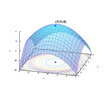
Minimization and maximization problems

Newton's method can be used to find a minimum or maximum of a function $f(x)$ . The derivative is zero at a minimum or maximum, so local minima and maxima can be found by applying Newton's method to the derivative. The iteration becomes:

x_{n+1}=x_{n}-{\frac {f'(x_{n})}{f''(x_{n})}}.

Multiplicative inverses of numbers and power series

An important application is Newton–Raphson division, which can be used to quickly find the reciprocal of a number, using only multiplication and subtraction.

Finding the reciprocal of $a$ amounts to finding the root of the function

f(x)=a-{\frac {1}{x}}

Newton's iteration is

{\begin{aligned}x_{n+1}&=x_{n}-{\frac {f(x_{n})}{f'(x_{n})}}\\&=x_{n}-{\frac {a-{\frac {1}{x_{n}}}}{\frac {1}{x_{n}^{2}}}}\\&=x_{n}(2-ax_{n})\end{aligned}}

Therefore, Newton's iteration needs only two multiplications and one subtraction.

This method is also very efficient to compute the multiplicative inverse of a power series.

Solving transcendental equations

Many transcendental equations can be solved using Newton's method. Given the equation

g(x)=h(x),

with $g (x)$ and/or $h (x)$ a transcendental function, one writes

f(x)=g(x)-h(x).

The values of $x$ that solve the original equation are then the roots of $f (x)$ , which may be found via Newton's method.

Obtaining zeros of special functions

Newton's method is applied to the ratio of Bessel functions in order to obtain its root.^[15]

Numerical verification for solutions of nonlinear equations

A numerical verification for solutions of nonlinear equations has been established by using Newton's method multiple times and forming a set of solution candidates.^[16]^[17]

Examples

Square root of a number

Consider the problem of finding the square root of a number. Newton's method is one of many methods of computing square roots.

For example, if one wishes to find the square root of 612, this is equivalent to finding the solution to

x^{2}=612

The function to use in Newton's method is then

f(x)=x^{2}-612

with derivative

f'(x)=2x.\,

With an initial guess of 10, the sequence given by Newton's method is

{\begin{matrix}x_{1}&=&x_{0}-{\dfrac {f(x_{0})}{f'(x_{0})}}&=&10-{\dfrac {10^{2}-612}{2\times 10}}&=&35.6\qquad \qquad \qquad \quad \;\,{}\\x_{2}&=&x_{1}-{\dfrac {f(x_{1})}{f'(x_{1})}}&=&35.6-{\dfrac {35.6^{2}-612}{2\times 35.6}}&=&{\underline {2}}6.395\,505\,617\,978\dots \\x_{3}&=&\vdots &=&\vdots &=&{\underline {24.7}}90\,635\,492\,455\dots \\x_{4}&=&\vdots &=&\vdots &=&{\underline {24.738\,6}}88\,294\,075\dots \\x_{5}&=&\vdots &=&\vdots &=&{\underline {24.738\,633\,753\,7}}67\dots \end{matrix}}

where the correct digits are underlined. With only a few iterations one can obtain a solution accurate to many decimal places.

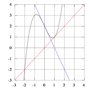
Solution of $cos x = x 3$

Consider the problem of finding the positive number $x$ with $cos x = x 3$ . We can rephrase that as finding the zero of $f (x) = cos(x) - x 3$ . We have $f' (x) = -sin(x) - 3 x 2$ . Since $cos(x) \leq 1$ for all $x$ and $x 3 > 1$ for $x > 1$ , we know that our solution lies between 0 and 1. We try a starting value of $x 0 = 0.5$ . (Note that a starting value of 0 will lead to an undefined result, showing the importance of using a starting point that is close to the solution.)

{\begin{matrix}x_{1}&=&x_{0}-{\dfrac {f(x_{0})}{f'(x_{0})}}&=&0.5-{\dfrac {\cos 0.5-0.5^{3}}{-\sin 0.5-3\times 0.5^{2}}}&=&1.112\,141\,637\,097\dots \\x_{2}&=&x_{1}-{\dfrac {f(x_{1})}{f'(x_{1})}}&=&\vdots &=&{\underline {0.}}909\,672\,693\,736\dots \\x_{3}&=&\vdots &=&\vdots &=&{\underline {0.86}}7\,263\,818\,209\dots \\x_{4}&=&\vdots &=&\vdots &=&{\underline {0.865\,47}}7\,135\,298\dots \\x_{5}&=&\vdots &=&\vdots &=&{\underline {0.865\,474\,033\,1}}11\dots \\x_{6}&=&\vdots &=&\vdots &=&{\underline {0.865\,474\,033\,102}}\dots \end{matrix}}

The correct digits are underlined in the above example. In particular, $x 6$ is correct to 12 decimal places. We see that the number of correct digits after the decimal point increases from 2 (for $x 3$ ) to 5 and 10, illustrating the quadratic convergence.

Pseudocode

The following is an example of an implementation of the Newton's Method for finding a root of a function f which has derivative fprime.

The initial guess will be $x 0 = 1$ and the function will be $f (x) = x 2 - 2$ so that $f' (x) = 2 x$ .

Each new iteration of Newton's method will be denoted by x1. We will check during the computation whether the denominator (yprime) becomes too small (smaller than epsilon), which would be the case if $f' (x n) \approx 0$ , since otherwise a large amount of error could be introduced.

%These choices depend on the problem being solved
x0 = 1 %The initial value
f = @(x) x^2 - 2 %The function whose root we are trying to find
fprime = @(x) 2*x %The derivative of f(x)
tolerance = 10^(-7) %7 digit accuracy is desired
epsilon = 10^(-14) %Don't want to divide by a number smaller than this

maxIterations = 20 %Don't allow the iterations to continue indefinitely
haveWeFoundSolution = false %Have not converged to a solution yet

for i = 1 : maxIterations

 y = f(x0)
 yprime = fprime(x0)

 if(abs(yprime) < epsilon) %Don't want to divide by too small of a number
 % denominator is too small
 break; %Leave the loop
 end

 x1 = x0 - y/yprime %Do Newton's computation

 if(abs(x1 - x0) <= tolerance * abs(x1)) %If the result is within the desired tolerance
 haveWeFoundSolution = true
 break; %Done, so leave the loop
 end

 x0 = x1 %Update x0 to start the process again

end

if (haveWeFoundSolution)
 ... % x1 is a solution within tolerance and maximum number of iterations
else
 ... % did not converge
end

Notes

↑ Wallis, John (1685). A Treatise of Algebra, both Historical and Practical. Shewing the Original, Progress, and Advancement thereof, from time to time, and by what Steps it hath attained to the Heighth at which it now is. Oxford: Richard Davis. doi:10.3931/e-rara-8842.
↑ Raphson, Joseph (1697). Analysis Æequationum Universalis seu ad Æequationes Algebraicas Resolvendas Methodus Generalis, & Expedita, Ex nova Infinitarum Serierum Methodo, Deducta ac Demonstrata (in Latin) (secunda ed.). London. doi:10.3931/e-rara-13516.
↑ "Accelerated and Modified Newton Methods".
↑ Ryaben'kii, Victor S.; Tsynkov, Semyon V. (2006), A Theoretical Introduction to Numerical Analysis, CRC Press, p. 243, ISBN 9781584886075 .
↑ Süli & Mayers 2003, Exercise 1.6
↑ Dence, Thomas (Nov 1997). "Cubics, chaos and Newton's method". Mathematical Gazette. 81: 403–408. doi:10.2307/3619617.
↑ Henrici, Peter (1974). "Applied and Computational Complex Analysis". 1.
↑ Strang, Gilbert (Jan 1991). "A chaotic search for $i$ ". The College Mathematics Journal. 22: 3–12. doi:10.2307/2686733.
↑ McMullen, Curt (1987). "Families of rational maps and iterative root-finding algorithms" (PDF). Annals of Mathematics. Second Series. 125 (3): 467–493. doi:10.2307/1971408.
↑ Rajkovic, Stankovic & Marinkovic 2002
↑ Press et al. 1992
↑ Stoer & Bulirsch 1980
↑ Zhang & Jin 1996
↑ Murota 1982
↑ Gil, Segura & Temme (2007)
↑ Kahan (1968)
↑ Krawczyk (1969)

References

Gil, A.; Segura, J.; Temme, N. M. (2007). Numerical methods for special functions (PDF). Society for Industrial and Applied Mathematics. ISBN 978-0-89871-634-4.
Süli, Endre; Mayers, David (2003). An Introduction to Numerical Analysis. Cambridge University Press. ISBN 0-521-00794-1.

External links

Hazewinkel, Michiel, ed. (2001) [1994], "Newton method", Encyclopedia of Mathematics, Springer Science+Business Media B.V. / Kluwer Academic Publishers, ISBN 978-1-55608-010-4
Weisstein, Eric W. "Newton's Method". MathWorld.
Newton's method, Citizendium.
Mathews, J., The Accelerated and Modified Newton Methods, Course notes.
Wu, X., Roots of Equations, Course notes.

This article is issued from Wikipedia. The text is licensed under Creative Commons - Attribution - Sharealike. Additional terms may apply for the media files.

[1] Wallis, John (1685). A Treatise of Algebra, both Historical and Practical. Shewing the Original, Progress, and Advancement thereof, from time to time, and by what Steps it hath attained to the Heighth at which it now is. Oxford: Richard Davis. doi:10.3931/e-rara-8842.

[2] Raphson, Joseph (1697). Analysis Æequationum Universalis seu ad Æequationes Algebraicas Resolvendas Methodus Generalis, & Expedita, Ex nova Infinitarum Serierum Methodo, Deducta ac Demonstrata (in Latin) (secunda ed.). London. doi:10.3931/e-rara-13516.

[3] "Accelerated and Modified Newton Methods".

[4] Ryaben'kii, Victor S.; Tsynkov, Semyon V. (2006), A Theoretical Introduction to Numerical Analysis, CRC Press, p. 243, ISBN 9781584886075 .

[5] Süli & Mayers 2003, Exercise 1.6

[6] Dence, Thomas (Nov 1997). "Cubics, chaos and Newton's method". Mathematical Gazette. 81: 403–408. doi:10.2307/3619617.

[7] Henrici, Peter (1974). "Applied and Computational Complex Analysis". 1.

[8] Strang, Gilbert (Jan 1991). "A chaotic search for $i$ ". The College Mathematics Journal. 22: 3–12. doi:10.2307/2686733.

[9] McMullen, Curt (1987). "Families of rational maps and iterative root-finding algorithms" (PDF). Annals of Mathematics. Second Series. 125 (3): 467–493. doi:10.2307/1971408.

[10] Rajkovic, Stankovic & Marinkovic 2002

[11] Press et al. 1992

[12] Stoer & Bulirsch 1980

[13] Zhang & Jin 1996

[14] Murota 1982

[15] Gil, Segura & Temme (2007)

[16] Kahan (1968)

[17] Krawczyk (1969)

Isaac Newton
Publications	De analysi per aequationes numero terminorum infinitas (1669, published 1711) Method of Fluxions (1671) De motu corporum in gyrum (1684) Philosophiæ Naturalis Principia Mathematica (1687) General Scholium (1713) Opticks (1704) The Queries (1704) Arithmetica Universalis (1707)
Other writings	Notes on the Jewish Temple Quaestiones quaedam philosophicae The Chronology of Ancient Kingdoms Amended (1728) An Historical Account of Two Notable Corruptions of Scripture (1754)
Discoveries and inventions	Calculus Fluxions Newton disc Newton polygon Newton–Okounkov body Newton's reflector Newtonian telescope Newton scale Newton's metal Newton's cradle Sextant
Theory expansions	Kepler's laws of planetary motion Problem of Apollonius
Newtonianism	Bucket argument Newton's inequalities Newton's law of cooling Newton's law of universal gravitation Post-Newtonian expansion Parameterized post-Newtonian formalism Newton–Cartan theory Schrödinger–Newton equation Gravitational constant Newton's laws of motion Newtonian dynamics Newton's method in optimization Gauss–Newton algorithm Truncated Newton method Newton's rings Newton's theorem about ovals Newton–Pepys problem Newtonian potential Newtonian fluid Classical mechanics Newtonian fluid Corpuscular theory of light Leibniz–Newton calculus controversy Newton's notation Rotating spheres Newton's cannonball Newton–Cotes formulas Newton's method Newton fractal Generalized Gauss–Newton method Newton's identities Newton polynomial Newton's theorem of revolving orbits Newton–Euler equations Newton number Kissing number problem Power number Newton's quotient Parallelogram of force Newton–Puiseux theorem Solar mass Dynamics Absolute space and time Absolute theory Finite difference Table of Newtonian series Impact depth Structural coloration Inertia Spectrum
Phrases	"Hypotheses non fingo" "Standing on the shoulders of giants"
Life	Cranbury Park Woolsthorpe Manor Early life Later life Religious views Occult studies The Mysteryes of Nature and Art Scientific revolution Copernican Revolution
Friends and family	Catherine Barton John Conduitt William Clarke Benjamin Pulleyn William Stukeley William Jones Isaac Barrow Abraham de Moivre John Keill
Cultural depictions	Newton (Blake) Newton (Paolozzi) In popular culture
Related	Writing of Principia Mathematica List of things named after Newton Isaac Newton Institute Isaac Newton Medal Isaac Newton Group of Telescopes Isaac Newton Telescope Newton (unit) Elements of the Philosophy of Newton Isaac Newton S/O Philipose

Root-finding algorithms
Bracketing (no derivative)	Bisection method
Quasi-Newton	False position Secant method
Newton	Newton's method
Hybrid methods	Brent's method
Polynomial methods	Bairstow's method Jenkins–Traub method