Fokas method

The Fokas method, or unified transform, is an algorithmic procedure for analysing boundary value problems for linear partial differential equations and for an important class of nonlinear PDEs belonging to the so-called integrable systems. It is named after Greek mathematician Athanassios S. Fokas.

Traditionally, linear boundary value problems are analysed using either integral transforms and infinite series, or by employing appropriate fundamental solutions.

Integral transforms and infinite series

For example, the Dirichlet problem of the heat equation on the half-line, i.e., the problem

$u_{t}=u_{xx},\quad 0<x<\infty ,\quad t>0,$

(Eq.1)

$u(x,0)=u_{0}(x),\quad 0<x<\infty ;\quad u(0,t)=g_{0}(t),\quad t>0,$

(Eq.2)

$u_{0}$ and $g_{0}$ given, can be solved via the sine-transform. The analogous problem on a finite interval can be solved via an infinite series. However, the solutions obtained via integral transforms and infinite series have several disadvantages:

1. The relevant representations are not uniformly convergent at the boundaries. For example, using the sine-transform, equations Eq.1 and Eq.2 imply

$u(x,t)={\frac {2}{\pi }}\int _{0}^{\infty }\sin(\lambda x)e^{-\lambda ^{2}t}\left[\int _{0}^{\infty }\sin(\lambda y)u_{0}(y)\,dy+\lambda \int _{0}^{t}e^{\lambda ^{2}\tau }g_{0}(\tau )\,d\tau \right]\,d\lambda .$

(Eq.3)

For $g_{0}(t)\neq 0$ , this representation cannot be uniformly convergent at $x=0$ , otherwise one could compute $u(0,t)$ by inserting the limit $x\rightarrow 0$ inside the integral of the rhs of Eq.3 and this would yield zero instead of $g_{0}(t)$ .

2. The above representations are unsuitable for numerical computations. This fact is a direct consequence of 1.

3. There exist traditional integral transforms and infinite series representations only for a very limited class of boundary value problems.
For example, there does not exist the analogue of the sine-transform for solving the following simple problem:

$u_{t}+u_{xxx}=0,\quad 0<x<\infty ,\quad t>0,$

(Eq.4)

supplemented with the initial and boundary conditions Eq.2.

For evolution PDEs, the Fokas method:

Constructs representations which are always uniformly convergent at the boundaries.
These representations can be used in a straightforward way, for example using MATLAB, for the numerical evaluation of the solution.
Constructs representations for evolution PDEs with spatial derivatives of any order.

In addition, the Fokas method constructs representations which are always of the form of the Ehrenpreis fundamental principle.

Fundamental solutions

For example, the solutions of the Laplace, modified Helmholtz and Helmholtz equations in the interior of the two-dimensional domain $\Omega$ , can be expressed as integrals along the boundary of $\Omega$ . However, these representations involve both the Dirichlet and the Neumann boundary values, thus since only one of these boundary values is known from the given data, the above representations are not effective. In order to obtain an effective representation, one needs to characterize the generalized Dirichlet to Neumann map; for example, for the Dirichlet problem one needs to obtain the Neumann boundary value in terms of the given Dirichlet datum.

For elliptic PDEs, the Fokas method:

Provides an elegant formulation of the generalised Dirichlet to Neumann map by deriving an algebraic relation, called the global relation, which couples appropriate transforms of all boundary values.
For simple domains and a variety of boundary conditions the global relation can be solved analytically. Furthermore, for the case that $\Omega$ is an arbitrary convex polygon, the global relation can be solved numerically in a straightforward way, for example using MATLAB. Furthermore, for the case that $\Omega$ is a convex polygon, the Fokas method constructs an integral representation in the Fourier complex plane. By using this representation together with the global relation it is possible to compute the solution numerically inside the polygon in a straightforward semi-analytic manner.

The forced heat equation on the half-line

Let $u(x,t)$ satisfy the forced heat equation

$u_{t}-u_{xx}=f(x,t),\ 0<x<\infty ,t>0,$

(Eq.5)

supplemental with the initial and boundary conditions Eq.2, where $g(t),\ u_{0}(x),\ f(x,t)$ are given functions with sufficient smoothness, which decay as $x\rightarrow \infty$ .

The unified transform involves the following three simple steps.

1. By employing the Fourier transform pair

{\widehat {f}}(\lambda )=\int _{0}^{\infty }e^{-i\lambda x}f(x)\,dx,\quad \operatorname {Im} \lambda \leq 0;

$f(x)={\frac {1}{2\pi }}\int _{-\infty }^{\infty }e^{i\lambda x}{\hat {f}}(\lambda )\,d\lambda ,\quad 0<x<\infty ,$

(Eq.6)

obtain the global relation.
For equation Eq.5, we find

$e^{\lambda ^{2}t}{\hat {u}}(\lambda ,t)=Q(\lambda ,t)-{\tilde {g_{1}}}(\lambda ^{2},t)-i\lambda {\tilde {g_{0}}}(\lambda ^{2},t),\quad \operatorname {Im} \lambda \leq 0,$

(Eq.7)

where the functions ${\hat {u}},\ Q,\ {\tilde {g_{1}}}$ and ${\tilde {g_{0}}}$ are the following integral transforms:

{\widehat {u}}(\lambda ,t)=\int _{0}^{\infty }e^{-i\lambda x}u(x,t)\,dx,\ \operatorname {Im} \lambda \leq 0,

Q(\lambda ,t)=\int _{0}^{\infty }e^{-i\lambda x}u_{0}(x)dx+\int _{0}^{t}\,d\tau \int _{0}^{\infty }dx\,e^{-i\lambda x+\lambda ^{2}\tau }f(x,\tau ),\quad \operatorname {Im} \lambda \leq 0,

${\tilde {g_{1}}}(\lambda ^{2},t)=\int _{0}^{t}e^{\lambda ^{2}\tau }u_{x}(0,\tau )\,d\tau ,\quad {\tilde {g_{0}}}(\lambda ^{2},t)=\int _{0}^{t}e^{\lambda ^{2}\tau }u(0,\tau )\,d\tau ,\quad \lambda \in \mathbb {C} .$

(Eq.8)

This step is similar with the first step used for the traditional transforms. However, equation Eq.7 involves the t-transforms of both $u(0,t)$ and $u_{x}(0,t)$ , whereas in the case of the sine-transform $u_{x}(0,t)$ does not appear in the analogous equation (similarly, in the case of the cosine-transform only $u_{x}(0,t)$ appears). On the other hand, equation Eq.7 is valid in the lower-half complex $\lambda$ -plane, wheres the analogous equations for the sine and cosine transforms are valid only for $\lambda$ real. The Fokas method is based on the fact that equation Eq.7 has a large domain of validity.

2. By using the inverse Fourier transform, the global relation yields an integral representation on the real line. By deforming the real axis to a contour in the upper half $\lambda$ -complex plane, it is possible to rewrite this expression as an integral along the contour $\partial D^{+}$ , where $\partial D^{+}$ is the boundary of the domain $D^{+}$ , which is the part of $D$ in the upper half complex $\lambda$ plane, with $D$ defined by

D:\{\lambda \in \mathbb {C} ,\ \Re \ \omega (\lambda )<0\},

where $\omega (\lambda )$ is defined by the requirement that $e^{i\lambda x+\omega (\lambda )t}$ solves the given PDE.

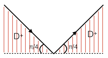Figure 1: The curve

\partial D^{+}

For equation Eq.5, equations Eq.6 and Eq.7 imply

$u(x,t)={\frac {1}{2\pi }}\int _{-\infty }^{\infty }e^{i\lambda x-\lambda ^{2}t}Q(\lambda ,t)\,d\lambda -{\frac {1}{2\pi }}\int _{\partial D^{+}}e^{i\lambda x-\lambda ^{2}t}[{\tilde {g_{1}}}(\lambda ^{2},t)+i\lambda {\tilde {g_{0}}}(\lambda ^{2},t)]\,d\lambda ,$

(Eq.9)

where the contour $\partial D^{+}$ is depicted in figure 1.

In this case, $\omega (\lambda )=-\lambda ^{2}=-|\lambda |^{2}e^{2i\theta }$ , where $\theta ={\rm {{arg}\lambda }}$ . Thus, $\Re \ \omega (k)<0$ implies $\sin 2\theta >0$ , i.e., $-{\frac {\pi }{4}}<\theta <{\frac {\pi }{4}}$ and ${\frac {3\pi }{4}}<\theta <{\frac {5\pi }{4}}$ .
The fact that the real axis can be deformed to $\partial D^{+}$ is a consequence of the fact that the relevant integral is an analytic function of $\lambda$ which decays in $D^{+}$ as $\lambda \rightarrow \infty$ .^[1]

3. By using the global relation and by employing the transformations in the complex- $\lambda$ plane which leave $\omega (\lambda )$ invariant, it is possible to eliminate from the integral representation of $u(x,t)$ the transforms of the unknown boundary values. For equation Eq.5, $\omega (\lambda )=\lambda ^{2}$ , thus the relevant transformation is $\lambda \rightarrow -\lambda$ . Using this transformation, equation Eq.7 becomes

$e^{\lambda ^{2}t}{\hat {u}}(-\lambda ,t)=Q(-\lambda ,t)-{\tilde {g_{1}}}(\lambda ^{2},t)+i\lambda {\tilde {g_{0}}}(\lambda ^{2},t),\quad \operatorname {Im} \lambda \geq 0.$

(Eq.10)

In the case of the Dirichlet problem, solving equation Eq.10 for ${\tilde {g_{1}}}$ and substituting the resulting expression in Eq.9 we find

$u(x,t)={\frac {1}{2\pi }}\int _{-\infty }^{\infty }e^{i\lambda x-\lambda ^{2}t}Q(\lambda ,t)\,d\lambda -{\frac {1}{2\pi }}\int _{\partial D^{+}}e^{i\lambda x-\lambda ^{2}t}[2i\lambda {\tilde {g_{0}}}(\lambda ^{2},t)+Q(-\lambda ,t)]\,d\lambda .$

(Eq.11)

If is important to note that the unknown term ${\hat {u}}(-\lambda ,t)$ does not contribute to the solution $u$ . Indeed, the relevant integral involves the term $e^{i\lambda x}{\hat {u}}(-\lambda ,t)$ , which is analytic and decays as $\lambda \rightarrow \infty$ in $D^{-}$ , thus Jordan's lemma implies that ${\hat {u}}(-\lambda ,t)$ yields a zero contribution.
Equation Eq.11 can be rewritten in a form which is consistent with the Ehrenpreis fundamental principle: if the boundary condition is specified for $0<\tau <T$ , where $T$ is a given positive constant, then using Cauchy's integral theorem, it follows that Eq.11 is equivalent with the following equation:

$u(x,t)={\frac {1}{2\pi }}\int _{-\infty }^{\infty }e^{i\lambda x-\lambda ^{2}t}Q(\lambda )\,d\lambda -{\frac {1}{2\pi }}\int _{\partial D^{+}}e^{i\lambda x-\lambda ^{2}t}[Q(-\lambda )+2i\lambda {\tilde {g_{0}}}(\lambda ^{2})]\,d\lambda ,$

(Eq.12)

where

Q(\lambda )={\widehat {u}}_{0}(\lambda )+\int _{0}^{\infty }dx\int _{0}^{T}dt\,e^{-i\lambda x+\lambda ^{2}t}f(x,t),

{\tilde {g_{0}}}(\lambda ^{2})=\int _{0}^{T}e^{\lambda ^{2}t}g_{0}(t)\,dt.

Uniform convergence
The unified transform constructs representations which are always uniformly convergent at the boundaries. For example, evaluating Eq.12 at $x=0$ , and then letting $\lambda \rightarrow -\lambda$ in the first term of the second integral in the rhs of (3.8), it follows that

u(0,t)=-{\frac {i}{\pi }}\int _{\partial D}e^{-\lambda ^{2}t}\lambda {\tilde {g_{0}}}(\lambda ^{2})\,d\lambda .

The change of variables $\lambda =e^{\frac {i\pi }{4}}{\sqrt {k}}$ , $k>0$ , implies that $u(0,t)=g(t)$ .

Numerical evaluation It is straightforward to compute the solution numerically. For simplicity we concentrate on the case that the relevant transforms can be computed analytically. For example,

f(x,t)=0,\ u_{0}(x)=e^{-a^{2}x},\ g_{0}(t)=\cos(bt),\ a,b,{\text{real constants}}.

Then, equation Eq.11 becomes

$2\pi u(x,t)=\int _{-\infty }^{\infty }{\frac {e^{i\lambda x-\lambda ^{2}t}}{i\lambda +a^{2}}}\,d\lambda -\int _{\partial D^{+}}e^{i\lambda x-\lambda ^{2}t}\left[{\frac {1}{-i\lambda +a^{2}}}+{\frac {i\lambda }{\lambda +ib}}{\bigl (}e^{(\lambda ^{2}+ib)t}-1{\bigr )}+{\frac {i\lambda }{\lambda -ib}}{\bigl (}e^{(\lambda ^{2}-ib)t}-1{\bigr )}\right]\,d\lambda .$

(Eq.13)

Figure 2: The contour L

For $\lambda$ on $\partial D^{+}$ , the term $e^{i\lambda x}$ decays exponentially as $|\lambda |\rightarrow \infty$ . Also by deforming $\partial D^{+}$ to $L$ where $L$ is a contour between the real axis and $\partial D^{+}$ , it follows that for $\lambda$ on $L$ the term $e^{-\lambda ^{2}t}$ also decays exponentially as $|\lambda |\rightarrow \infty$ . Thus, equation Eq.13 becomes

$2\pi u(x,t)=\int _{L}\left\{e^{i\lambda x-\lambda ^{2}t}\left[{\frac {1}{i\lambda +a^{2}}}+{\frac {1}{i\lambda -a^{2}}}\right]+i\lambda e^{i\lambda x}\left[{\frac {e^{ibt}-e^{-\lambda ^{2}t}}{\lambda +ib}}+{\frac {e^{-ibt}-e^{-\lambda ^{2}t}}{\lambda -ib}}\right]\right\}\,d\lambda ,$

and the rhs of the above equation can be computed using MATLAB.
An Evolution Equation with Spatial Derivatives of Arbitrary order.
Suppose that $e^{i\lambda x+\omega (\lambda )t}$ is a solution of the given PDE. Then, $\partial D^{+}$ is the boundary of the domain $D^{+}$ defined earlier.

If the given PDE contain spatial derivatives of order $n$ , then for $n$ even, the global relation involves ${\frac {n}{2}}$ unknowns, whereas for $n$ odd it involves $(n+1)/2$ or $(n-1)/2$ unknowns (depending on the coefficient of the highest derivative). However, using an appropriate number of transformations in the complex $\lambda$ -plane which leave $\omega (\lambda )$ invariant, it is possible to obtain the needed number of equations, so that the transforms of the unknown boundary values can be obtained in terms of ${\hat {u}}$ and of the given boundary data in terms of the solution of a system of algebraic equations.

The Laplace equation in the interior of a polygon

The transformations $z=x+iy,\ {\bar {z}}=x-iy,$ imply

${\frac {\partial }{\partial z}}={\frac {1}{2}}\left({\frac {\partial }{\partial x}}-i{\frac {\partial }{\partial y}}\right),\quad {\frac {\partial }{\partial {\bar {z}}}}={\frac {1}{2}}\left({\frac {\partial }{\partial x}}+i{\frac {\partial }{\partial y}}\right).$

(Eq.14)

Hence,

{\frac {\partial ^{2}}{\partial z\,\partial {\bar {z}}}}={\frac {1}{4}}\left({\frac {\partial ^{2}}{\partial x^{2}}}+{\frac {\partial ^{2}}{\partial y^{2}}}\right).

Thus, the Laplace equation

$u_{xx}+u_{yy}=0,$

(Eq.15)

can be written in the form

$u_{z{\bar {z}}}=0.$

(Eq.16)

Hence, $u$ satisfies the Laplace equation Eq.15 if and only if the function $u_{z}$ is analytic.
The global relation

Suppose that $u$ satisfies the Laplace equation in the two dimensional bounded domain $\Omega$ . Then, the function $u_{z}$ and hence $u_{z}e^{-i\lambda z}$ are analytic in $\Omega$ , thus, Cauchy's integral theorem implies the global relation

$\int _{\partial \Omega }e^{-i\lambda z}u_{z}(z)\,dz=0,\quad \lambda \in \mathbb {C} ,$

(Eq.17)

where $\partial \Omega$ denotes the boundary of $\Omega$ . An alternative global relation is given by

$\int _{\partial \Omega }e^{-i\lambda z}\left({\frac {\partial u}{\partial w}}+\lambda u{\frac {dz}{ds}}\right)\,ds,\quad \lambda \in \mathbb {C} ,$

(Eq.18)

where ${\frac {\partial u}{\partial w}}$ denotes the derivative of $u$ along the normal to the curve $\partial\Omega$ in the outward derivative, and $s$ denotes the arclength of the curve $\partial \Omega$ .

The Dirichlet to Neumann map for a convex polygon

Suppose that $\Omega$ is the interior of a bounded convex polygon specified by the corners $z_{1},z_{2},\dots \ z_{n}$ . In this case, the global relation Eq.17 takes the form

$\sum _{j=1}^{n}u_{j}(\lambda )=0,\ \lambda \in \mathbb {C} ,$

(Eq.19)

where

$u_{j}(\lambda )={\frac {1}{2}}\int _{z_{j}}^{z_{j}+1}e^{-i\lambda z}(u_{x}-iu_{y})\,dz,$

(Eq.20)

or

$u_{j}(\lambda )=\int _{z_{j}}^{z_{j}+1}e^{-i\lambda z}\left({\frac {\partial u}{\partial w}}+\lambda u{\frac {dz}{ds}}\right)\,ds.$

(Eq.21)

The side $S_j$ , which is the side between $z_{j}$ and $z_{{j+1}}$ , can be parametrized by

z(t)=m_{j}+th_{j},\ m_{j}={\frac {z_{j}+z_{j+1}}{2}},\ h_{j}={\frac {z_{j+1}-z_{j}}{2}},\ t\in [-1,1].

Hence,

ds=|h_{j}|\,dt,\ dz=h_{j}\,dt.

The functions $u$ and ${\frac {\partial u}{\partial w}}$ can be approximated in terms of Legendre polynomials:

$u^{j}(t)\approx \sum _{\ell =0}^{N-1}a_{\ell }^{j}P_{\ell }(t),\quad {\frac {\partial u^{j}(t)}{\partial w}}\approx \sum _{\ell =0}^{N-1}b_{\ell }^{j}P_{\ell }(t),$

(Eq.22)

where for the cases of the Dirichlet, or the Neamann, or the Robin boundary value problems, either $a_{\ell }^{j}$ , or $b_{\ell }^{j}$ , or a linear combination of $a_{\ell }^{j}$ and $b_{\ell }^{j}$ , is given.

Equation Eq.19 now becomes an approximate global relation, where

$u_{j}(\lambda )=\sum _{\ell =0}^{N-1}e^{-im_{j}\lambda }(b_{\ell }^{j}|h_{j}|+\lambda a_{\ell }^{j}h_{j}){\widehat {P}}_{\ell }(\lambda h_{j}),\ \lambda \in \mathbb {C} ,$

(Eq.23)

with ${\hat {P}}_{\ell }(\lambda )$ denoting the Fourier transform of $P_{\ell }(t)$ , i.e.,

${\widehat {P}}_{\ell }(\lambda )=\int _{-1}^{1}e^{-i\lambda t}P_{\ell }(t)\,dt,\quad \lambda \in \mathbb {C} .$

(Eq.24)

${\hat {P}}_{\ell }(\lambda )$ can be computed numerically via ${\hat {P}}_{\ell }(\lambda )={\frac {\sqrt {-2i\pi \lambda }}{-i\lambda }}I_{\ell +{\frac {1}{2}}}(-i\lambda ),$ where $I_{\ell }$ denotes the modified Bessel function of the first kind.

The global relation involves $N$ unknown constants (for the Dirichlet problem, these constants are $b_{\ell }^{j}$ ). By evaluating the global relation at a sufficiently large number of different values of $\lambda$ , the unknown constants can be obtained via the solution of a system of algebraic equations.

It is convenient to chose the above values of $\lambda$ on the $n$ rays $-{\bar {h}}_{j}\rho ,\ \rho >0,\ j=1,\dots ,n.$ For this choice, as $|\lambda |\rightarrow \infty$ , the relevant system is diagonally dominant, thus its condition number is very small.^[2]

References

↑ Deconinck, B.; Trogdon, T.; Vasan, V. (2014-01-01). "The Method of Fokas for Solving Linear Partial Differential Equations". SIAM Review. 56 (1): 159–186. doi:10.1137/110821871. ISSN 0036-1445.
↑ Hashemzadeh, P.; Fokas, A. S.; Smitheman, S. A. (2015-03-08). "A numerical technique for linear elliptic partial differential equations in polygonal domains". Proc. R. Soc. A. 471 (2175): 20140747. doi:10.1098/rspa.2014.0747. ISSN 1364-5021. PMC 4353048. PMID 25792955.

This article is issued from Wikipedia. The text is licensed under Creative Commons - Attribution - Sharealike. Additional terms may apply for the media files.

[1] Deconinck, B.; Trogdon, T.; Vasan, V. (2014-01-01). "The Method of Fokas for Solving Linear Partial Differential Equations". SIAM Review. 56 (1): 159–186. doi:10.1137/110821871. ISSN 0036-1445.

[2] Hashemzadeh, P.; Fokas, A. S.; Smitheman, S. A. (2015-03-08). "A numerical technique for linear elliptic partial differential equations in polygonal domains". Proc. R. Soc. A. 471 (2175): 20140747. doi:10.1098/rspa.2014.0747. ISSN 1364-5021. PMC 4353048. PMID 25792955.