Legendre polynomials

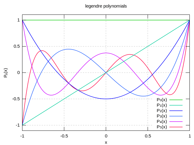The six first Legendre polynomials.

In mathematics, Legendre polynomials (named after Adrien-Marie Legendre) are the polynomial solutions $P_n(x)$ to Legendre's differential equation

${\frac {\mathrm {d} }{\mathrm {d} x}}\left[\left(1-x^{2}\right){\frac {\mathrm {d} P_{n}(x)}{\mathrm {d} x}}\right]+n(n+1)P_{n}(x)=0\,.$

(1)

with integer parameter $n\geq 0$ and with the convention $P_{n}(1)=1$ . The $P_n(x)$ form a polynomial sequence of orthogonal polynomials of degree n. They can be expressed using Rodrigues' formula:

P_{n}(x)={\frac {1}{2^{n}n!}}{\frac {\mathrm {d} ^{n}}{\mathrm {d} x^{n}}}\left(x^{2}-1\right)^{n}\,,

or any of the other representations given below.

The differential equation admits another, non-polynomial solution, the Legendre functions of the second kind $Q_{n}$ , discussed below. A two-parameter generalization of (Eq. 1) is called Legendre's general differential equation, solved by the Associated Legendre polynomials. Legendre functions are solutions of Legendre's differential equation (generalized or not) with non-integer parameters.

Legendre's differential equation is frequently encountered in physics and other technical fields. In particular, it occurs when solving Laplace's equation (and related partial differential equations) in spherical coordinates. The generating function is the basis for multipole expansions.

Recursive definition

The Legendre differential equation may be solved using the standard power series method. The equation has regular singular points at $x = \pm1$ so, in general, a series solution about the origin will only converge for $| x | < 1$ . When $n$ is an integer, the solution $P n (x)$ that is regular at $x = 1$ is also regular at $x = -1$ , and the series for this solution terminates (i.e. it is a polynomial).

$P n$ can also be defined as the coefficients in a Taylor series expansion of the generating function^[1]

${\frac {1}{\sqrt {1-2xt+t^{2}}}}=\sum _{n=0}^{\infty }P_{n}(x)t^{n}\,.$

(2)

Expanding the Taylor series in Eq. 2 for the first two terms gives

P_{0}(x)=1\,,\quad P_{1}(x)=x

for the first two Legendre polynomials. To obtain further terms without resorting to direct expansion of the Taylor series, Eq. 2 is differentiated with respect to $t$ on both sides and rearranged to obtain

{\frac {x-t}{\sqrt {1-2xt+t^{2}}}}=\left(1-2xt+t^{2}\right)\sum _{n=1}^{\infty }nP_{n}(x)t^{n-1}\,.

Replacing the quotient of the square root with its definition in Eq. 2, and equating the coefficients of powers of $t$ in the resulting expansion gives Bonnet’s recursion formula

(n+1)P_{n+1}(x)=(2n+1)xP_{n}(x)-nP_{n-1}(x)\,.

This relation, along with the first two polynomials $P 0$ and $P 1$ , allows the Legendre polynomials to be generated recursively.

Explicit representations

Explicit representations include

{\begin{aligned}P_{n}(x)&={\frac {1}{2^{n}}}\sum _{k=0}^{n}{\binom {n}{k}}^{2}(x-1)^{n-k}(x+1)^{k}\\P_{n}(x)&=\sum _{k=0}^{n}{\binom {n}{k}}{\binom {n+k}{k}}\left({\frac {x-1}{2}}\right)^{k}\\P_{n}(x)&={\frac {1}{2^{n}}}\sum _{k=0}^{[{\frac {n}{2}}]}(-1)^{k}{\binom {n}{k}}{\binom {2n-2k}{n}}x^{n-2k}\\P_{n}(x)&=2^{n}\sum _{k=0}^{n}x^{k}{\binom {n}{k}}{\binom {\frac {n+k-1}{2}}{n}}\,,\end{aligned}}

where the last, which is immediate from the recursion formula, expresses the Legendre polynomials by simple monomials and involves the multiplicative formula of the binomial coefficient.

The first few Legendre polynomials are:

{\begin{array}{r|r}n&P_{n}(x)\\\hline 0&1\\1&x\\2&{\tfrac {1}{2}}\left(3x^{2}-1\right)\\3&{\tfrac {1}{2}}\left(5x^{3}-3x\right)\\4&{\tfrac {1}{8}}\left(35x^{4}-30x^{2}+3\right)\\5&{\tfrac {1}{8}}\left(63x^{5}-70x^{3}+15x\right)\\6&{\tfrac {1}{16}}\left(231x^{6}-315x^{4}+105x^{2}-5\right)\\7&{\tfrac {1}{16}}\left(429x^{7}-693x^{5}+315x^{3}-35x\right)\\8&{\tfrac {1}{128}}\left(6435x^{8}-12012x^{6}+6930x^{4}-1260x^{2}+35\right)\\9&{\tfrac {1}{128}}\left(12155x^{9}-25740x^{7}+18018x^{5}-4620x^{3}+315x\right)\\10&{\tfrac {1}{256}}\left(46189x^{10}-109395x^{8}+90090x^{6}-30030x^{4}+3465x^{2}-63\right)\\\hline \end{array}}

The graphs of these polynomials (up to $n = 5$ ) are shown below:

Orthogonality

An important property of the Legendre polynomials is that they are orthogonal with respect to the $L 2$ norm on the interval $-1 \leq x \leq 1$ :

\int _{-1}^{1}P_{m}(x)P_{n}(x)\,\mathrm {d} x={\frac {2}{2n+1}}\delta _{mn}

(where $δ mn$ denotes the Kronecker delta, equal to 1 if $m = n$ and to 0 otherwise).

In fact, an alternative derivation of the Legendre polynomials is by carrying out the Gram–Schmidt process on the polynomials ${1, x, x 2, ...}$ with respect to this inner product. The reason for this orthogonality property is that the Legendre differential equation can be viewed as a Sturm–Liouville problem, where the Legendre polynomials are eigenfunctions of a Hermitian differential operator:

{\frac {\mathrm {d} }{\mathrm {d} x}}\left(\left(1-x^{2}\right){\frac {\mathrm {d} }{\mathrm {d} x}}P(x)\right)=-\lambda P(x)\,,

where the eigenvalue $λ$ corresponds to $n (n + 1)$ .

Applications of Legendre polynomials

Expanding a 1/r potential

The Legendre polynomials were first introduced in 1782 by Adrien-Marie Legendre^[2] as the coefficients in the expansion of the Newtonian potential

{\frac {1}{\left|\mathbf {x} -\mathbf {x} '\right|}}={\frac {1}{\sqrt {r^{2}+{r'}^{2}-2r{r'}\cos \gamma }}}=\sum _{l=0}^{\infty }{\frac {{r'}^{l}}{r^{l+1}}}P_{l}(\cos \gamma )

where $r$ and $r'$ are the lengths of the vectors $x$ and $x'$ respectively and $γ$ is the angle between those two vectors. The series converges when $r > r'$ . The expression gives the gravitational potential associated to a point mass or the Coulomb potential associated to a point charge. The expansion using Legendre polynomials might be useful, for instance, when integrating this expression over a continuous mass or charge distribution.

Legendre polynomials occur in the solution of Laplace's equation of the static potential, $\nabla 2 Φ (x) = 0$ , in a charge-free region of space, using the method of separation of variables, where the boundary conditions have axial symmetry (no dependence on an azimuthal angle). Where $ẑ$ is the axis of symmetry and $θ$ is the angle between the position of the observer and the $ẑ$ axis (the zenith angle), the solution for the potential will be

\Phi (r,\theta )=\sum _{l=0}^{\infty }\left(A_{l}r^{l}+B_{l}r^{-(l+1)}\right)P_{l}(\cos \theta )\,.

$A l$ and $B l$ are to be determined according to the boundary condition of each problem.^[3]

They also appear when solving the Schrödinger equation in three dimensions for a central force.

Legendre polynomials in multipole expansions

Legendre polynomials are also useful in expanding functions of the form (this is the same as before, written a little differently):

{\frac {1}{\sqrt {1+\eta ^{2}-2\eta x}}}=\sum _{k=0}^{\infty }\eta ^{k}P_{k}(x)

which arise naturally in multipole expansions. The left-hand side of the equation is the generating function for the Legendre polynomials.

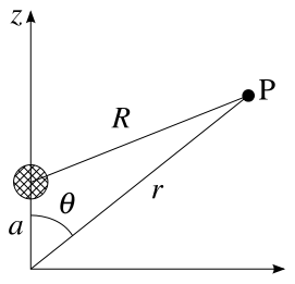
As an example, the electric potential $Φ (r, θ)$ (in spherical coordinates) due to a point charge located on the $z$ -axis at $z = a$ (see diagram right) varies as

\Phi (r,\theta )\propto {\frac {1}{R}}={\frac {1}{\sqrt {r^{2}+a^{2}-2ar\cos \theta }}}

If the radius $r$ of the observation point $P$ is greater than $a$ , the potential may be expanded in the Legendre polynomials

\Phi (r,\theta )\propto {\frac {1}{r}}\sum _{k=0}^{\infty }\left({\frac {a}{r}}\right)^{k}P_{k}(\cos \theta )

where we have defined $η = a / r < 1$ and $x = cos θ$ . This expansion is used to develop the normal multipole expansion.

Conversely, if the radius $r$ of the observation point $P$ is smaller than $a$ , the potential may still be expanded in the Legendre polynomials as above, but with $a$ and $r$ exchanged. This expansion is the basis of interior multipole expansion.

Legendre polynomials in trigonometry

The trigonometric functions $cos nθ$ , also denoted as the Chebyshev polynomials $T n (cos θ) \equiv cos nθ$ , can also be multipole expanded by the Legendre polynomials $P n (cos θ)$ . The first several orders are as follows:

{\begin{aligned}T_{0}(\cos \theta )&=&1&=&P_{0}(\cos \theta )\\T_{1}(\cos \theta )&=&\cos \theta &=&P_{1}(\cos \theta )\\T_{2}(\cos \theta )&=&\cos 2\theta &=&{\tfrac {1}{3}}{\bigl (}4P_{2}(\cos \theta )-P_{0}(\cos \theta ){\bigr )}\\T_{3}(\cos \theta )&=&\cos 3\theta &=&{\tfrac {1}{5}}{\bigl (}8P_{3}(\cos \theta )-3P_{1}(\cos \theta ){\bigr )}\\T_{4}(\cos \theta )&=&\cos 4\theta &=&{\tfrac {1}{105}}{\bigl (}192P_{4}(\cos \theta )-80P_{2}(\cos \theta )-7P_{0}(\cos \theta ){\bigr )}\\T_{5}(\cos \theta )&=&\cos 5\theta &=&{\tfrac {1}{63}}{\bigl (}128P_{5}(\cos \theta )-56P_{3}(\cos \theta )-9P_{1}(\cos \theta ){\bigr )}\\T_{6}(\cos \theta )&=&\cos 6\theta &=&{\tfrac {1}{1155}}{\bigl (}2560P_{6}(\cos \theta )-1152P_{4}(\cos \theta )-220P_{2}(\cos \theta )-33P_{0}(\cos \theta ){\bigr )}\end{aligned}}

Another property is the expression for $sin (n + 1) θ$ , which is

{\frac {\sin(n+1)\theta }{\sin \theta }}=\sum _{l=0}^{n}P_{l}(\cos \theta )P_{n-l}(\cos \theta )

Additional properties of Legendre polynomials

Legendre polynomials are symmetric or antisymmetric, that is^[4]

P_{n}(-x)=\left(-1\right)^{n}P_{n}(x)\,.

Another useful property is

\int _{-1}^{1}P_{n}(x)\,\mathrm {d} x=0

for

n\geq 1

,

which follows from considering the orthogonality relation with $P_{0}(x)=1$ . It is convenient when a Legendre series $\sum _{i}a_{i}P_{i}$ is used to approximate a function or experimental data: the average of the series over the interval -1...1 is simply given by the leading expansion coefficient $a_{0}$ .

Since the differential equation and the orthogonality property are independent of scaling, the Legendre polynomials' definitions are "standardized" (sometimes called "normalization", but note that the actual norm is not 1) by being scaled so that

P_{n}(1)=1\,.

The derivative at the end point is given by

P_{n}'(1)={\frac {n(n+1)}{2}}\,.

The Askey–Gasper inequality for Legendre polynomials reads

\sum _{j=0}^{n}P_{j}(x)\geq 0\,\quad {\text{for }}x\geq -1\,.

A sum of Legendre polynomials is related to the Dirac delta function for $-1 \leq y \leq 1$ and $-1 \leq x \leq 1$

\delta (y-x)={\frac {1}{2}}\sum _{l=0}^{\infty }(2l+1)P_{l}(y)P_{l}(x)\,.

The Legendre polynomials of a scalar product of unit vectors can be expanded with spherical harmonics using

P_{l}\left(r\cdot r'\right)={\frac {4\pi }{2l+1}}\sum _{m=-l}^{l}Y_{lm}(\theta ,\phi )Y_{lm}^{*}(\theta ',\phi ')\,,

where the unit vectors $r$ and $r'$ have spherical coordinates $(θ, φ)$ and $(θ', φ')$ , respectively.

Recursion relations

As discussed above, the Legendre polynomials obey the three-term recurrence relation known as Bonnet’s recursion formula

(n+1)P_{n+1}(x)=(2n+1)xP_{n}(x)-nP_{n-1}(x)

and

{\frac {x^{2}-1}{n}}{\frac {\mathrm {d} }{\mathrm {d} x}}P_{n}(x)=xP_{n}(x)-P_{n-1}(x)\,.

Useful for the integration of Legendre polynomials is

(2n+1)P_{n}(x)={\frac {\mathrm {d} }{\mathrm {d} x}}{\bigl (}P_{n+1}(x)-P_{n-1}(x){\bigr )}\,.

From the above one can see also that

{\frac {\mathrm {d} }{\mathrm {d} x}}P_{n+1}(x)=(2n+1)P_{n}(x)+{\bigl (}2(n-2)+1{\bigr )}P_{n-2}(x)+{\bigl (}2(n-4)+1{\bigr )}P_{n-4}(x)+\cdots

or equivalently

{\frac {\mathrm {d} }{\mathrm {d} x}}P_{n+1}(x)={\frac {2P_{n}(x)}{\left\|P_{n}\right\|^{2}}}+{\frac {2P_{n-2}(x)}{\left\|P_{n-2}\right\|^{2}}}+\cdots

where $| | P n | |$ is the norm over the interval $-1 \leq x \leq 1$

\|P_{n}\|={\sqrt {\int _{-1}^{1}{\bigl (}P_{n}(x){\bigr )}^{2}\,\mathrm {d} x}}={\sqrt {\frac {2}{2n+1}}}\,.

Asymptotes

Asymptotically for $l \to \infty$ for arguments in (-1, 1)

{\begin{aligned}P_{l}(\cos \theta )&=J_{0}(l\theta )+{\mathcal {O}}\left(l^{-1}\right)\\&={\frac {2}{\sqrt {2\pi l\sin \theta }}}\cos \left(\left(l+{\tfrac {1}{2}}\right)\theta -{\frac {\pi }{4}}\right)+{\mathcal {O}}\left(l^{-1}\right)\end{aligned}}

and for arguments of magnitude greater than 1

{\begin{aligned}P_{l}\left({\frac {1}{\sqrt {1-e^{2}}}}\right)&=I_{0}(le)+{\mathcal {O}}\left(l^{-1}\right)\\&={\frac {1}{\sqrt {2\pi le}}}{\frac {(1+e)^{\frac {l+1}{2}}}{(1-e)^{\frac {l}{2}}}}+{\mathcal {O}}\left(l^{-1}\right)\,,\end{aligned}}

where $J 0$ and $I 0$ are Bessel functions.

Legendre polynomials with transformed argument

Shifted Legendre polynomials

The shifted Legendre polynomials are defined as

{\tilde {P}}_{n}(x)=P_{n}(2x-1)\,

.

Here the "shifting" function $x \mapsto 2 x - 1$ is an affine transformation that bijectively maps the interval $[0,1]$ to the interval $[-1,1]$ , implying that the polynomials $P̃ n (x)$ are orthogonal on $[0,1]$ :

\int _{0}^{1}{\tilde {P}}_{m}(x){\tilde {P}}_{n}(x)\,\mathrm {d} x={\frac {1}{2n+1}}\delta _{mn}\,.

An explicit expression for the shifted Legendre polynomials is given by

{\tilde {P}}_{n}(x)=(-1)^{n}\sum _{k=0}^{n}{\binom {n}{k}}{\binom {n+k}{k}}(-x)^{k}\,.

The analogue of Rodrigues' formula for the shifted Legendre polynomials is

{\tilde {P}}_{n}(x)={\frac {1}{n!}}{\frac {\mathrm {d} ^{n}}{\mathrm {d} x^{n}}}\left(x^{2}-x\right)^{n}\,.

The first few shifted Legendre polynomials are:

{\begin{array}{r|r}n&{\tilde {P}}_{n}(x)\\\hline 0&1\\1&2x-1\\2&6x^{2}-6x+1\\3&20x^{3}-30x^{2}+12x-1\\4&70x^{4}-140x^{3}+90x^{2}-20x+1\\5&252x^{5}-630x^{4}+560x^{3}-210x^{2}+30x-1\end{array}}

Legendre rational functions

The Legendre rational functions are a sequence of orthogonal functions on [0, ∞). They are obtained by composing the Cayley transform with Legendre polynomials.

A rational Legendre function of degree n is defined as:

R_{n}(x)={\frac {\sqrt {2}}{x+1}}\,P_{n}\left({\frac {x-1}{x+1}}\right)\,.

They are eigenfunctions of the singular Sturm-Liouville problem:

(x+1)\partial_x(x\partial_x((x+1)v(x)))+\lambda v(x)=0

with eigenvalues

\lambda _{n}=n(n+1)\,.

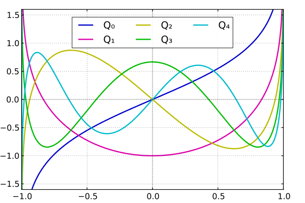
Legendre functions of the second kind ( $Q n$ )

As well as polynomial solutions, the Legendre equation has non-polynomial solutions represented by infinite series. These are the Legendre functions of the second kind, denoted by $Q n (x)$ .

Q_{n}(x)={\frac {n!}{1\cdot 3\cdots (2n+1)}}\left(x^{-(n+1)}+{\frac {(n+1)(n+2)}{2(2n+3)}}x^{-(n+3)}+{\frac {(n+1)(n+2)(n+3)(n+4)}{2\cdot 4(2n+3)(2n+5)}}x^{-(n+5)}+\cdots \right)

The differential equation

{\frac {\mathrm {d} }{\mathrm {d} x}}\left(\left(1-x^{2}\right){\frac {\mathrm {d} }{\mathrm {d} x}}f(x)\right)+n(n+1)f(x)=0

has the general solution

f(x)=AP_{n}(x)+BQ_{n}(x)

,

where $A$ and $B$ are constants.

Notes

↑ Arfken & Weber 2005, p.743
↑ Legendre, A.-M. (1785) [1782]. "Recherches sur l'attraction des sphéroïdes homogènes". Mémoires de Mathématiques et de Physique, présentés à l'Académie Royale des Sciences, par divers savans, et lus dans ses Assemblées (PDF) (in French). X. Paris. p. 411–435. Archived from the original (PDF) on 2009-09-20.
↑ Jackson, J. D. (1999). Classical Electrodynamics (3rd ed.). Wiley & Sons. p. 103. ISBN 978-0-471-30932-1.
↑ Arfken & Weber 2005, p.753

References

Abramowitz, Milton; Stegun, Irene Ann, eds. (1983) [June 1964]. "Chapter 8". Handbook of Mathematical Functions with Formulas, Graphs, and Mathematical Tables. Applied Mathematics Series. 55 (Ninth reprint with additional corrections of tenth original printing with corrections (December 1972); first ed.). Washington D.C.; New York: United States Department of Commerce, National Bureau of Standards; Dover Publications. pp. 332, 773. ISBN 978-0-486-61272-0. LCCN 64-60036. MR 0167642. LCCN 65-12253. See also chapter 22.
Arfken, George B.; Weber, Hans J. (2005). Mathematical Methods for Physicists. Elsevier Academic Press. ISBN 0-12-059876-0.
Bayin, S. S. (2006). Mathematical Methods in Science and Engineering. Wiley. ch. 2. ISBN 978-0-470-04142-0.
Belousov, S. L. (1962). Tables of Normalized Associated Legendre Polynomials. Mathematical Tables. 18. Pergamon Press. ISBN 978-0-08-009723-7.
Courant, Richard; Hilbert, David (1953). Methods of Mathematical Physics. 1. New York, NY: Interscience. ISBN 978-0-471-50447-4.
Dunster, T. M. (2010), "Legendre and Related Functions", in Olver, Frank W. J.; Lozier, Daniel M.; Boisvert, Ronald F.; Clark, Charles W., NIST Handbook of Mathematical Functions, Cambridge University Press, ISBN 978-0521192255, MR 2723248
El Attar, Refaat (2009). Legendre Polynomials and Functions. CreateSpace. ISBN 978-1-4414-9012-4.
Koornwinder, Tom H.; Wong, Roderick S. C.; Koekoek, Roelof; Swarttouw, René F. (2010), "Orthogonal Polynomials", in Olver, Frank W. J.; Lozier, Daniel M.; Boisvert, Ronald F.; Clark, Charles W., NIST Handbook of Mathematical Functions, Cambridge University Press, ISBN 978-0521192255, MR 2723248

External links

A quick informal derivation of the Legendre polynomial in the context of the quantum mechanics of hydrogen
Hazewinkel, Michiel, ed. (2001) [1994], "Legendre polynomials", Encyclopedia of Mathematics, Springer Science+Business Media B.V. / Kluwer Academic Publishers, ISBN 978-1-55608-010-4
Wolfram MathWorld entry on Legendre polynomials
Dr James B. Calvert's article on Legendre polynomials from his personal collection of mathematics
The Legendre Polynomials by Carlyle E. Moore
Legendre Polynomials from Hyperphysics

This article is issued from Wikipedia. The text is licensed under Creative Commons - Attribution - Sharealike. Additional terms may apply for the media files.

[1] Arfken & Weber 2005, p.743

[2] Legendre, A.-M. (1785) [1782]. "Recherches sur l'attraction des sphéroïdes homogènes". Mémoires de Mathématiques et de Physique, présentés à l'Académie Royale des Sciences, par divers savans, et lus dans ses Assemblées (PDF) (in French). X. Paris. p. 411–435. Archived from the original (PDF) on 2009-09-20.

[3] Jackson, J. D. (1999). Classical Electrodynamics (3rd ed.). Wiley & Sons. p. 103. ISBN 978-0-471-30932-1.

[4] Arfken & Weber 2005, p.753